@include "lib.awk"
@include "sdiscrete.awk"
"""
Simple Rule Generation (with `bore`)
------------------------------------
`Bore` is an ultra-simple rule generator for generating ultra-simple
rules. Why am I `bore`-ing you about `bore`?
Machine learners generate modes. Sometimes, people read those models.
What kind of learners generate the kind of models that people want to
read?
Before answering that, consider the plight of the modern business
manager. For 21st-century businesses, the problem is not accessing
data but ignoring irrelevant data. Most modern businesses can elec-
tronically access mountains of data such as transactions for the past
two years or the state of their assembly line. The trick is effec-
tively using the available data. In practice, this means summarizing
large data sets to find the _diamonds in the dust_ - that is, the data
that really matters.
In the data mining community, "learning the least" is an uncommon
goal. Most data miners are zealous hunters seeking detailed summaries
and generating extensive and lengthy descriptions. Here, we take a
different approach and assume that busy people don't need- or can't
use- complex models. Rather, they want only the data they need to
achieve the most benefits.
An Aside
--------
Formally, `bore` is a greedy search for rules, guided by a Bayesian
ranking heuristic. Rather than ranking features, `bore` ranks feature
ranges.
But described like that, `bore` does not seem very interesting. The
real important thing about `bore` is not the simplicity of the
algorith. Rather, it is its connection to cognitive psychology.
`Bore` is an extreme form of Occam's Razor. This is an idea first
expressed by William of Ockham (c. 1287 - 1347). It is a principle of
parsimony for problem-solving. It states that among competing
hypotheses, the one with the fewest assumptions should be selected.
To put that another way:
+ Prune the unnecessary;
+ Focus on what's left.
It turns out that Occam's razor is a core principle of cognitive
psychology. In the early 1980s, Jill Larkin and her colleagues
explained human expertise in terms of a long term memory of
possibilities and a short term memory for the things we are currently
considering.
+ Expert and novice performance in solving physics problems
J Larkin, J McDermott, DP Simon, HA Simon ,
Science, Vol. 208, pp. 1335-1342.
According to Larkin et al. novices confuse themselves by overloading
their short term memory. They run so many "what if" queries that their
short term memory chokes and dies. Experts, on the other hand, only
reason about the things that matter so their short term memories have
space for conclusions. The exact details of how this is done is quite
technical, but the main lesson is clear:
+ Experts are experts since they _know what to ignore_.
Occam's razor has obvious business implications. For one thing, we can
build better decision support systems:
+ In 1916, Henri Fayol said that managers plan, organise, co-ordinate
and control. In that view, managers systematically assessing all
relevant factors to generate some optimum plan.
+ Fayol, Henri. 1916. Administration
industrielle et generale; prevoyance, organisation,
commandement, coordination, controle. H. Dunod et E. Pinat,
Paris, OCLC 40204128.
+ Then in the sixties, computers were used to automatically and
routinely generate the information needed for the Fayol model. This
was the era of the management information system (MIS), where thick
wads of paper were routninely filed in the trash can.
+ Ackoff, R. L. 1967. "Management Misinformation Systems."
Management Science (December): 319331.
+ In 1975, Mintzberg's classic empirical fly-on-the-wall tracking of
managers in the day-to-day work demonstrated that the Fayol model was
normative, rather than descriptive. For example, Mintzberg found 56
U.S. foreman who averaged 583 activities in an eight-hour shift (one
every 48 seconds). Another study of 160 British middle and top
managers found that they worked for half an hour or more without
interruption only once every two days.
+ Mintzberg, H. 1975. "The Manager's Job: Folklore and
Fact." Harvard Business Review (July August):
29-61.
The lesson of MIS is that management decision making is not inhibited
by a lack of information. Rather, according to Ackoff, it is confused
by an excess of irrelevant information. This was true in the sixties
and now, in the age of the Internet, it is doubly true. As Mitch Kapor
said in his famous quote:
+ _Getting information off the Internet is like taking a drink from a fire hydrant._
Further, the lesson of Mintzberg's study is that it is vitally
important to give managers _succinct_ summaries of their available
actions since, given their work pressures, they just cannot digest
long and overly-complex ideas. Too much data can overload a decision
maker with too many irrelevancies. Data must be condensed, before it
is useful for supporting decisions. Modern decision-support systems
evolved to filter useless information to deliver small amounts of
relevant information (a subset of all information) to the manager.
Enter Ockam's razor and `bore`
How it works
------------
`Bore` is short for "best or rest". Given two tables, it sorts feature
ranges according to their frequency in the two tables. `Bore` ranks
highest the ranges that are more common in the _better_ table.
Note that `bore` does not care how you decided which table was
_better_ (that is something you can discuss with your business users).
However it is defined, `bore` seeks some constraint that when applied
to the data in both tables, that it selects more for _better_ than for
worse.
`Bore` uses a variant of Bayes theorem to sort the ranges. For
example, in K = 10, 000 examples fall into two tables containing 1,000
examples in _best_ and 9,000 in _rest. Suppose further we were
ranking the value of requiring very high reliability; i.e. _rely =
vh_. If so, we would count how often it appears in the _best_ and
_rest_ tables. For this example, we will assume it appears 10 times
in _best_ and 5 times in _rest_. Hence, we could score this range as
follows:
E = (rely=vh)
P(best) = 1000/10000 = 0.1
freq(E|best) = 10/1000 = 0.01
freq(E|rest) = 5/9000 = 0.00056
b = like(best|E) = freq(E|best) * P(best) = 0.001
r = like(rest|E) = freq(E|rest) * P(rest) = 0.000504
P(best|E) = b/(b + r) = 0.66
Clark explored this approach and found it to be a poor ranking
heuristic when it is distracted by low frequeny evidence. For
example, note how the probability of _E_ belonging to the _best_ class
is moderately high even though its _support_ is very low; i.e. _P
(best|E) = 0.66_ but _freq(E|best) = 0.01_.
+ _R. Clark. Faster treatment learning, Computer Science, Portland State University. Master's thesis, 2005_
To avoid such unreliable low frequency evidence, Clark augmented the
above with a support term. Support should increase as the frequency
of a range increases, i.e. _like(best|x)_ is a valid support measure.
Hence `bore` ranks ranges via
P(best|E) * support(best|E) = b^2 / (b+r)
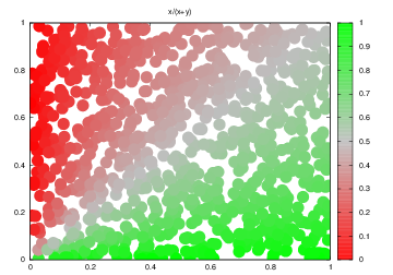
This simple equation has some interesting properties. The range of _b_
and _r_ are zero to one. Here's _ b / (b+r)_. Note how this function
can reward ranges, even if they are very uncommon in _b_:
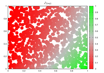
And here's _b^2 / (b+r)_. Note that this measure offers enthusiastic
support for only the ranges that are frequent in _b_.
Code
----
### Main Driver
Note that this main driver divided numerics into _bins=7_.
Here's an example main driver for `bore`:
+ It defines _better_ to be the class _tested negative_ in the file _data/diabetes.csv_ (so the goal here is to find the
things that selects for patients that are more _negative_ (i.e. not sick) than _positive_ (i.e. sick).
+ It reads some data from disk into a take (see `readcsv`);
+ It discretizes the numerics (see `sdiscrete`):
+ How the data is discretized is a lower-level detail that we need obsess on at this time.
+ For the record, we use `bins=7` and ignore any
division whose `max - min` is less than `tiny=0.3` times the standard deviation for that column.
+ But you could use something else.
+ It then ranks the discretized ranges use the `bore` function.
+ It then tests that ranking using the `forwardSelect` described below.
Code follows:
"""
function _bore( _Table, f,t1,bins,tiny,
want,_Tables,t,out,enough,some,best,m,good,skip) {
f="data/diabetes.csv";
bins = 7; tiny=0.3; enough=0.25; want="tested_negative"
readcsv(f,0,_Table)
t1 = sdiscrete(_Table, 0, bins, tiny)
tables(_Table[t1],_Tables)
m=bore(_Tables,names,want,enough,good,skip)
o(colnum[t1],"nums")
o(good,"good")
forwardSelect(length(datas[want]),-1,1,m,
names,want,good,_Tables,best)
o(best,"best")
}
"""
### Range Ranking with `bore`
Note that in the following, we employ a couple of search biases:
+ The following two rules come from the geometry of _b^2 / (b+r)_ space (shown above):
+ *Rule1*: Only consider ranges with _b > r_;
+ *Rule2*: Only consider ranges with _b>0.5_;
+ *Rule3*: Ignore all ranges with a score less than _enough*max(score)_ (in this code, _enough=25%);
"""
function bore(_Tables,all,want,enough,out,skip,
t,yes,no,best,rest,x,y,b,r,tmp,max,inc,m,items) {
for(t in all) {
items = length(datas[t])
t == want ? best += items : rest += items
for(x in indeps[t])
if(! (x in skip))
for(y in counts[t][x]) {
inc = counts[t][x][y]
t == want ? yes[x][y] += inc : no[x][y] += inc
}}
for(x in yes)
for(y in yes[x]) {
b = yes[x][y]/ best
r = no[ x][y]/ rest
if (b > r && b > 0.5) { # rule1 and rule2
m++
out[m]["x"] = x
out[m]["y"] = y
out[m]["z"] = tmp = b^2/(b+r)
if (tmp > max) max=tmp
}}
for(m in out)
if (out[m]["z"] < enough*max) # rule3
delete out[m]
return asort(out,out,"zsortdown")
}
"""
### Checking Ranges with `forwardSelect`
While the _bore_ heuristic can suggest what _might_ be useful, it
is important to check those suggestions with a _forward select_.
+ Take the ranges, sorted by the _b^2/(b+r)
+ Find the rows selected by the top _x_ items in that sort.
+ Score those rows.
+ Let _best_ be the rows with the _want_ed class
+ Let _rest_ be the rest
+ Let score be _best/(best + rest)_
+ Note some termination rules:
+ *Rule1*: Give up if _enough_ of the _best_ (here , _enough_ = 33%);
+ *Rule2*: Give up if the top _x_ items do not better than the top _x-1_ items;
+ *Rule3*: Give up if we run out of good ranges
this If they contain the _wanted_ class, then _best++_.
+ Recurse on the se
+ Find the rows selected by the top _x+1_ items.
+ If the
"""
function forwardSelect(seen,b4,lo,hi,all,want,good,_Tables,out,support,
t,m,total,score,some,tmp,best,rest) {
support = support ? support : 0.33
support = support * length(datas[want])
if (lo > hi) return somes(good,lo-1,out) # Rule3
if (seen < support) return somes(good,lo-1,out) # Rule1
somes(good,lo,some)
for(t in all) { # for `all` the tables we are examining
tmp = rowsWith(some,_Tables[t])
t == want ? best += tmp : rest += tmp
}
score = best/(best+rest)
print "Got", best,int(100*score),"%"
if (best > support && score > b4) # Rule1, Rule2
return forwardSelect(best,score,lo+1,hi,all,want,good,_Tables,out)
else
return somes(good,lo-1,out)
}
"""
Not shown here is `rowsWith`. This is function that takes
a list of the top _x_ ranges and finds the right rows.
Here's the relevant code, copied from
[tables.awk](https://github.com/timm/auk/blob/master/src/table.auk):
In this code `this` contains the top _x_ items.
The `rowsWith` function finds all the rows that match to the `this`.
function rowsWith(this,_Table, out, d) {
for(d in data)
if (rowHas(this,data[d]))
out[d]
return length(out)
}
This code uses `rowHas` to match to one specific row.
Note that `rowHas` has to handle conjunctions and disjunctions.
So:
+ *Rule1*: for each column mentioned in `this`, there must be
at least of those ranges in the row.
Note that this rule handles disjunctions and conjunctions in a uniform
manner.
+ If `this` reference some column multiple times, we must find
its range at least once.
+ And if `this` only mentions one range for a column, then
it still works.
Code:
function rowHas(this,row, col,val,has) {
for(col in this) {
for(val in this[col])
if (row[col]== val)
has[col]++
if (has[col]<1) return 0 # Rule1
}
return 1
}
### Low-level Detail: Select `some`
Here's a small function that explores `all` known ranges, then returns
just `some` (specifically, only up to the first `max` items in `all`).
"""
function somes(all,max,some, i,x,y) {
for(i=1;i<=max;i++) {
x = all[i]["x"]
y = all[i]["y"]
some[x][y]
}}
"""
## Results
Now that all that is working, lets see some output on
[data/diabtes.csv](https://github.com/timm/auk/blob/master/data/diabetes.csv).
In this example, the column names are numbered as follows:
nums[age] = (8)
nums[insu] = (5)
nums[mass] = (6)
nums[pedi] = (7)
nums[plas] = (2)
nums[preg] = (1)
nums[pres] = (3)
nums[skin] = (4)
### Ranges Ranked with `Bore`
Here is what `bore` things are promising ranges, ranked according
to their `bore` score (shown here as `z`).
The first entry is about column five (insu: use of insulin).
Note that `bore` has decided that _<=120.857_ is the best predictor
for _testedNegative_.
good[1]
| [x] = (5)
| [y] = (<=120.857)
| [z] = (0.450894)
good[2]
| [x] = (7)
| [y] = (<=0.669143)
| [z] = (0.450441)
good[3]
| [x] = (8)
| [y] = (<=34.2857)
| [z] = (0.438954)
good[4]
| [x] = (1)
| [y] = (<=2.42857)
| [z] = (0.326694)
Exercise for the reader: why are there only four entries in this list?
Surely there are many more ranges in _diabestes.csv_?
### Ranges Selected by `forwardSelect`:
`ForwardSelect` tried the first one, the two, then three,
then four items in the above list. It found that the first
three were as good with anything else.
best[5]
| [<=120.857] = ()
best[7]
| [<=0.669143] = ()
best[8]
| [<=34.2857] = ()
To read the above, recall that
+ Column 8 = age
+ Column 5 = insu (use of insulin)
+ Column 7 = pedi (the diabtes pedigree function). The Diabetes
Pedigree Function (DPF) was developed by Smith, et al. [4] to
provide a synthesis of the diabetes mellitus history in relatives
and the genetic relationship of those relatives to the subject. The
DPF uses information from parents, grandparents, siblings, aunts and
uncles, and first cousins. It provides a measure of the expected
genetic influence of affected and unaffected relatives on the
subject’s eventual diabetes risk.
+ J. W. Smith, J. E. Everhart, W. C. Dickson, W. C. Knowler,
and R. S. Johannes (1988). Using the ADAP learning algorithm to
forecast the onset of diabetes mellitus. InSymposium on Computer
Applications in Medical Care, 261–265.
## Discussion
The result above is interesting: out of all that data, there is
only a few ranges that most predict for (say) not having diabetes.
This is a repeated result with `bore`. If features are discretized
and then ranked by `b^2/(b+r)` and we ignore all ranges the _b < r_
or _b < 0.5_, we end up with very small rule bases. This suggests
that either `bore` is missing details OR that the underlying
model in these data sets is very simple.
In support of the latter idea (that the underlying structures in many
data sets are very simple), I offer the follow range ranking result
using a completely different method. In this approach, the
wider the horizontal line, the more a range can select for different
classes (to the left selects for defective software classes
and to the right selects for non-defective). Also, the closer
the ranges to the vertical line, the less useful they are for
selecting for any class. Note that most of the ranges are very
narrow and fall close to the vertical line; i.e. only a very small
subset of these ranges matter at all.

I show the above, not because I endorse that particular analysis
(it does not have a `forwardSelect` so it can offer overly enthusiastic
support for things that do not actually work). But rather,
I show it to illustrate that the methods of many researchers report
that when doing range selection, only a few things matter.
Coming back to the start of this lecture- note how we can now
offer automatic support for
+ Prune the unnecessary
+ Focus on what's left.
(By the way, if you want to know how that last diagram was generated,
see
+ [Nomograms for Visualization of Naive Bayesian Classifier](http://iccle.googlecode.com/svn/trunk/share/pdf/mozina04.pdf).
M. Mozina and J. Demsar and M. Kattan and B. Zupa,
Proceedings PKDD'04, 2004)
### Cautionary Note
Of course, not all domains are so simple as to allow the extraction
of ultra-simple rules. I'm often asked "how to check if this approach
is too simple?". My reply is "try it" using a cross-val experiment.
All the above code runs in near-linear time:
+ If the resulting rules
work then you have an ultra-simple solution.
+ And if they don't, then at least you'll have some a simple
baseline result against which you can document the power of
your favorite, more sophisticated technique.
"""