Data mining is extracting pearls from historical data.
When data is absent, we don't mine. Instead, we farm.
Knowledge farming is a three stage process:
Our case study will be software process design. Using our method, a set of minimal recommendations are highly specialized to a specific software project will be developed.
That is, after recording what is known in a model, that model should be validated, explored using simulations, then summarized to find the key factors that most improve model behavior.
Many general tools and methodologies exist for modeling such as:
Note that for software process programming, elaborate new modeling paradigms may not be required. For example, the Little-JIL process programming language just uses standard programming constructs such as pre-conditions, post-conditions, exception handlers, and a top-down decomposition tree showing sub-tasks inside tasks.
Simulations can be based on nominal or off-nominal values. Nominal simulations draw their inputs from known operational profiles of system inputs. Off-nominal monte-carlo (also called stochastic) simulations, where inputs are selected at random, can check for unanticipated situations. Stochastic simulation has been extensively applied to models of software process.
In a sensitivity analysis, the key factors that most influence a model are isolated. Also, recommended settings for those key factors are generated. We take care to distinguish sensitivity analysis from traditional optimization methods. In our experience, the real systems we deal with are so complex that they do not always fit into (e.g.) a linear optimization framework. Studying data grown from simulators lets us investigate complex, non-linear systems using a variety of data driven distributions. These models can capture complex feedback and rework loops which are not possible for traditional optimization methods. Our experience is that simulation models can look at processes in detail as well as at a high level of abstraction which is where the more analytic models must reside. Finally, simulation models can capture multiple performance measures not able to be explored using these optimization formulations. This is not to say that traditional optimization models are not useful. For certain questions, traditional optimization formulations provide the best fit for the question that is trying to be answered. However, for many questions, the standard optimization models are not the best choice and something like the learners discussed below may be more useful.
Many researchers have predicated their work on the truism that catching errors during early software life cycle is very important. For example, the first author has written:
Is this general truism true is specific cases? Well...
The model for this case study originally developed in 1995 By Dr. David Raffo (PSU) and subsequently tailored to a specific large-scale development project at a leading software development firm with the following properties:
A high-level block diagram of this model is shown below The model is far more complex that suggested by this figure since each block references many variables shared by all other blocks.
The model is really two models:
The discrete event model contained 30+ process steps with two levels of hierarchy. The main performance measures of development cost, product quality and project schedule were computed by the model. These performance measures could also be recorded for any individual process step as desired. Some of the inputs to the simulation model included productivity rates for various processes; the volume of work (i.e. KSLOC); defect detection and injection rates for all phases; effort allocation percentages across all phases of the project; rework costs across all phases; parameters for process overlap; the amount / effect of training provided; and resource constraints.
Actual data were used for model parameters where possible. For example, inspection data was collected from individual inspection forms for the two past releases of the product. Distributions for defect detection rates and inspection effectiveness where developed from these individual inspection reports. Also, effort and schedule data were collected from the corporate project management tracking system. Lastly, senior developers and project managers were surveyed and interviewed to obtain values for other project parameters when hard data were not available.
Models were developed from this data using multiple regression to predict defect rates and task effort. The result was a model that predicted the three main performance measures of cost, quality, and schedule. A list of all of the process modification supported by the model are too numerous to list here. Suffice to say that small to medium scope process changes could be easily incorporated and tested using the model.
For each phase of the modeled process, there was a choice of either having one of four inspection types;
TR(a,b,c)
The outputs of the model are assessed via a multi-attribute utility function:
 utility =  40*(14 - quality) +
           320*(70 - expense) +
           640*(24 - duration)
where quality, expense and duration are defined as follows. Quality is the number of major defects (i.e. severity 1 and 2) estimated to remain in the product when released to customers. Expense is the number of person-months of effort used to perform the work on the project and to implement the changes to the process that were studied. Duration is the number of calendar months for the project from the beginning of functional specification until the product was released to customers.
This function was created after extensive debriefing of the business users who funded the development of this model.
The baseline simulation model of the life cycle development process was validated in a number of ways. The most important of which were as follows:
The simulation model described above contains four phases of development and four inspection types at each phase. The four phases were functional specification (FS); high level design (HLD); low level design (LLD); and coding (CODE). The four inspection types were full Fagan, baseline, walk through, and none.
This results in $4^4$ different configurations:NNNN, NNNF, NNNB, NNNW, NNFN, NNFF, ..., etc. Each configuration was executed 50 times, resulting in 50*4^4=12800 runs. Each run was summarized using the utility equation.
The results were passed to the data mining team in a WINDOWS EXCEL spreadsheet that required some pre-processing.
Note that, in the following, all the lines starting looking like this:
% COM
are bash commands. In practice, I DON'T type these in at the command line. Rather, I place them in a bash script file. This makes re-running things easier. FYI: in developing the following, I must have re-run things dozens of times.
If you want to see that script, go look at http://www.cs.pdx.edu/~timm/dm/inspectprep. The following notes explain that script.
 % . config
 % a=${tmp}a
 % b=${tmp}b
 % ./dos2unix  $1 > $a
 NNNN,n,0,2,0,0,0,0,0,0,0,n,0,...
     ,n,0,0,5,0,0,0,0,0,0,n,0....
     ,n,0,0,0,0,0,7,0,8,0,n,0....
 ....
 NNNF,n,1,0,0,0,4,0,0,0,9,n,0....
     ,n,0,a,0,c,0,0,0,0,0,n,0....
That is, a blank first field means ``same as the above''.
So we need to remove lines 1,2,3 and copy down the policy symbol into the blank fields on line one
% $gawk 'NR>4' $a | $gawk -F, -f inspectprep.awk > $b
 #inspectprep.awk
 $1 {type=$1}
   {str=type;
    for(i=2;i<=NF;i++) str=str "," $i;
    print str;
   }
zapblanks $b > $a
quality, expense and
duration figures used in the utility calculations were
removed (otherwise the learner just generates a trite
theory reproducing the utility equations):
% cut -d, -f"1-41,47-60" $a > $b
Cut is a handy UNIX utility for pulling columns. For more details,
see
http://www.mcsr.olemiss.edu/cgi-bin/man-cgi?cut+1
 getnames() {
        names=`$gawk -F, 'NR==4 {OFS=",";
                    for(I=1;I<=NF;I++) $I=  "_" $I "_" I
                    print $0}' $a`
        echo $names
        exit
  }
% getnames
We trap the output of this function into the names variable:
  names="policy,_spec_2,_specDist_3,_specv1_4,_specv2_5,_specv3_6,_specStaff_7,_detCap_8"
  names="$names,_inspEff_9,_inspDur_10,_corErr_11,_hidesign_12,_hiDist_13,_hidesignv1_14"
  names="$names,_hidesignv2_15,_hidesignv3_16,_hiStaff_17,_detCap_18,_inspEff_19,_inspDur_20"
  names="$names,_corErr_21,_lodesign_22,_loDist_23,_lodesignv1_24,_lodesignv2_25,_lodesignv3_26"
  names="$names,_loStaff_27,_detCap_28,_inspEff_29,_inspDur_30,_corErr_31,_code_32,_codeDist_33"
  names="$names,_codev1_34,_codev2_35,_codev3_36,_codeStaff_37,_detCap_38,_inspEff_39,_inspDur_40"
  names="$names,_corErr_41,_inspEff_48"
  names="$names,_inspDur_49,_corErr_50,_inspEff_52,_inspDur_53,_inspEff_54,_inspDur_55,_inspEff_56"
  names="$names,_inspDur_57,_inspEff_58,_inspDur_59,utility"
 % ranges -n"$names"   -a -d $b > data/inspectn.arff
 % bars -1 6 -r 1000 $b > inspectn.bars
This generates information like the following. At this point, its good to show the domain experts the ranges files (to check if there are any madness in the data). The ranges are as follows:
 @RELATION "/tmp/3615b"
 @ATTRIBUTE policy {BBBB,BFFF,BNNB,BNNF,BNNN,BNNW,...
 @ATTRIBUTE _spec_2 {b,f,n,w}
 @ATTRIBUTE _specDist_3 {0,tr}
 @ATTRIBUTE _specv1_4 {0,0.07,0.35,0.3927}
 @ATTRIBUTE _specv2_5 {0,0.15,0.5,0.561}
 @ATTRIBUTE _specv3_6 {0,0.23,0.65,0.7293}
 @ATTRIBUTE _specStaff_7 {0,1,6}
The bar graph showing the ranges of the utilities is as follows:
  3000|   2|
  4000|   3|
  5000|   9| *
  6000|  30| ****
  7000|  63| *********
  8000| 119| ****************
  9000| 210| ****************************
 10000| 273| *************************************
 11000| 296| ****************************************
 12000| 181| ************************
 13000|  88| ************
 14000|  23| ***
 15000|   3|
data/inspectn.arff is now ready for data mining
using learners that can process numeric classes. In order
to pass the same data to discrete class data miners,
we need to discretize the class values. We do this using
three percentile chops
(using
http://www.cs.pdx.edu/~timm/dm/percentile.html),
then calling ranges again
to get all the values for our learning file.
 % percentile -b 3 $b > $a
 % ranges -n"$names"  -a -d $a > data/inspectd.arff
Ranges also prints the boundary positions of the percentile
chops:
 1 9483.116
 2 10985.467
 3 14643.515
That is:
 if utility < 10987 then class1
 else if if < 14642 then class2
      else class3
How many items fall into each class? Well:
% bars -r0 $a
 class1| 865| ****************************************
 class2| 433| ********************
 class3|   2|
Hmmm... not ideal. This is nearly a two class problem. So why did we use these boundaries that produces chops of such different sizes? Well, we experimented with different chops found that these 3 chops gave us best accuracies:
 33% correct with 7 chops
 60% correct with 4 chops
 80% correct with 3 chops
The file data/inspectd.arff is now ready for data mining
using learners that can process discrete classes.
 % percentile -b 5 $b > $a
 % ranges -n"$names"  $a > inspectn.data
 % cp $a  inspectd.data
The range boundaries are:
 1 8656.582
 2 9842.604
 3 10698.390
 4 11664.238
 5 14755.164
That is:
 if utility < 9843 then class1
 else if utility < 10698 then class2
      else if utility < 11664 then class3
           else if utility < 14755 then class4
                else class5
How many items fall into each class? Well:
% bars -r0 inspectd.data
 class1| 519| ****************************************
 class2| 260| ********************
 class3| 260| ********************
 class4| 260| ********************
 class5|   1|
That solo class5 will muck up treatment learning since due to the minimal best support over-fitting bias avoidance technique of TAR3. So we manually delete that one class5 example.
TAR3 also needs a configuration file:
% cat inspectd.cfg
 maxSize:        4
 randomTrials:   50
 futileTrials:   5
 granularity:    7
 maxNumber:      50
 bestClass:      20%
Anyway, the files inspectd.cfg, inspectd.names and inspectd.data are now ready for data mining using learners that can process discrete classes.
 #Instances:          1299
 #Numeric attributes:   27
 #Discrete attributes:  25
 #Discrete classes:      2 (for J48)
                         4 (for TAR3)
           | run time |                     | theory size
 learner   |  MIN:SEC | ACC | CORR   | LIFT | (#chars)
 ----------+----------+-----+--------+------+-------------
 TAR3           1:11                   2.35       21
 LSR            1:53          0.7447            1365
 Trees:
    Regression  1:51          0.7526            1538
    Model       3:18          0.7418             627
    Decision    0:23     81%                    1953
Notes:
SIZE number was calculated by taking the output theories shown above, removing all spaces,
then doing a character count:
gawk '{gsub(/[ \t]*/,""); print $0}' text | wc -c
Much learning, little meaning. The following theory has a correlation of 0.7447 but is opaque (at least to me):
 utility = 7370
           + 1220policy=WNNN,NWNN,FNNW,FNNB,BNNN,NNWN,NNNW,WNNW,BNNW,WNNB,BNNB,WWWW,NNNB,NNWW,FNNF,NNWB,NNFN,BNNF,WNNF,NNWF,BBBB,FFFF,NNNF,BFFF
           + 258policy=FNNB,BNNN,NNWN,NNNW,WNNW,BNNW,WNNB,BNNB,WWWW,NNNB,NNWW,FNNF,NNWB,NNFN,BNNF,WNNF,NNWF,BBBB,FFFF,NNNF,BFFF
           + 640policy=NNWN,NNNW,WNNW,BNNW,WNNB,BNNB,WWWW,NNNB,NNWW,FNNF,NNWB,NNFN,BNNF,WNNF,NNWF,BBBB,FFFF,NNNF,BFFF
           + 505policy=NNNW,WNNW,BNNW,WNNB,BNNB,WWWW,NNNB,NNWW,FNNF,NNWB,NNFN,BNNF,WNNF,NNWF,BBBB,FFFF,NNNF,BFFF
           - 190policy=WNNW,BNNW,WNNB,BNNB,WWWW,NNNB,NNWW,FNNF,NNWB,NNFN,BNNF,WNNF,NNWF,BBBB,FFFF,NNNF,BFFF
           + 206policy=BNNB,WWWW,NNNB,NNWW,FNNF,NNWB,NNFN,BNNF,WNNF,NNWF,BBBB,FFFF,NNNF,BFFF
           - 177policy=WWWW,NNNB,NNWW,FNNF,NNWB,NNFN,BNNF,WNNF,NNWF,BBBB,FFFF,NNNF,BFFF
           + 890policy=NNNB,NNWW,FNNF,NNWB,NNFN,BNNF,WNNF,NNWF,BBBB,FFFF,NNNF,BFFF
           - 296policy=NNWW,FNNF,NNWB,NNFN,BNNF,WNNF,NNWF,BBBB,FFFF,NNNF,BFFF
           + 545policy=NNFN,BNNF,WNNF,NNWF,BBBB,FFFF,NNNF,BFFF
           + 640policy=WNNF,NNWF,BBBB,FFFF,NNNF,BFFF
           + 459policy=NNWF,BBBB,FFFF,NNNF,BFFF - 143policy=BBBB,FFFF,NNNF,BFFF
           + 835policy=NNNF,BFFF - 142_spec_2=n,b + 27_spec_2=b + 3690_detCap_8
           - 135_inspEff_9 - 7320_inspDur_10 - 64400_corErr_11 - 760_detCap_18
           - 134_inspEff_19 - 7310_inspDur_20 - 64300_corErr_21 - 9100_detCap_28
           - 134_inspEff_29 - 7320_inspDur_30 - 64300_corErr_31 + 6170_detCap_38
           - 134_inspEff_39 - 7320_inspDur_40 - 64400_corErr_41
           + 21500_inspEff_48 + 1.17e6_inspDur_49 + 64400_corErr_50
Here's another opaque theory with a correlation of 0.7447 but it is still meaningless (at least to me):
 policy=NNFN,BNNF,WNNF,NNWF,BBBB,FFFF,NNNF,BFFF <= 0.5 :
 |   policy=NNWN,NNNW,WNNW,BNNW,WNNB,BNNB,WWWW,NNNB,NNWW,FNNF,NNWB,NNFN,BNNF,WNNF,NNWF,BBBB,FFFF,NNNF,BFFF <= 0.5 :
 |   |   policy=WNNN,NWNN,FNNW,FNNB,BNNN,NNWN,NNNW,WNNW,BNNW,WNNB,BNNB,WWWW,NNNB,NNWW,FNNF,NNWB,NNFN,BNNF,WNNF,NNWF,BBBB,FFFF,NNNF,BFFF <= 0.5 :
 |   |   |   _detCap_8 <= 0.431 : LM1 (60/116%)
 |   |   |   _detCap_8 >  0.431 : LM2 (40/82.8%)
 |   |   policy=WNNN,NWNN,FNNW,FNNB,BNNN,NNWN,NNNW,WNNW,BNNW,WNNB,BNNB,WWWW,NNNB,NNWW,FNNF,NNWB,NNFN,BNNF,WNNF,NNWF,BBBB,FFFF,NNNF,BFFF >  0.5 :
 |   |   |   _detCap_8 <= 0.491 :
 |   |   |   |   _inspDur_10 <= 94 : LM3 (120/83%)
 |   |   |   |   _inspDur_10 >  94 : LM4 (31/115%)
 |   |   |   _detCap_8 >  0.491 : LM5 (99/102%)
 |   policy=NNWN,NNNW,WNNW,BNNW,WNNB,BNNB,WWWW,NNNB,NNWW,FNNF,NNWB,NNFN,BNNF,WNNF,NNWF,BBBB,FFFF,NNNF,BFFF >  0.5 :
 |   |   policy=BNNB,WWWW,NNNB,NNWW,FNNF,NNWB,NNFN,BNNF,WNNF,NNWF,BBBB,FFFF,NNNF,BFFF <= 0.5 : LM6 (250/81.6%)
 |   |   policy=BNNB,WWWW,NNNB,NNWW,FNNF,NNWB,NNFN,BNNF,WNNF,NNWF,BBBB,FFFF,NNNF,BFFF >  0.5 : LM7 (300/76.9%)
 policy=NNFN,BNNF,WNNF,NNWF,BBBB,FFFF,NNNF,BFFF >  0.5 :
 |   policy=NNWF,BBBB,FFFF,NNNF,BFFF <= 0.5 :
 |   |   _detCap_38 <= 0.418 : LM8 (65/74.5%)
 |   |   _detCap_38 >  0.418 : LM9 (85/58.1%)
 |   policy=NNWF,BBBB,FFFF,NNNF,BFFF >  0.5 :
 |   |   _corErr_50 <= 155 : LM10 (169/74.5%)
 |   |   _corErr_50 >  155 :
 |   |   |   policy=NNNF,BFFF <= 0.5 : LM11 (41/42.4%)
 |   |   |   policy=NNNF,BFFF >  0.5 :
 |   |   |   |   _detCap_38 <= 0.519 : LM12 (15/56.1%)
 |   |   |   |   _detCap_38 >  0.519 : LM13 (25/42.6%)
     LM1:  utility = 6940
     LM2:  utility = 8180
     LM3:  utility = 8780
     LM4:  utility = 7860
     LM5:  utility = 9320
     LM6:  utility = 9750
     LM7:  utility = 10300
     LM8:  utility = 10700
     LM9:  utility = 11400
     LM10:  utility = 11900
     LM11:  utility = 12400
     LM12:  utility = 12500
     LM13:  utility = 13600
The model tree learner generated one linear model with a correlation of 0.7418
 LM1 (1300/82.5%)
 LM1:  utility = 7290
                 + 1360policy=WNNN,NWNN,FNNW,FNNB,BNNN,NNWN,NNNW,WNNW,BNNW,WNNB
                              ,BNNB,WWWW,NNNB,NNWW,FNNF,NNWB,NNFN,BNNF,WNNF,NNWF
                              ,BBBB,FFFF,NNNF,BFFF
                 + 612policy=NNWN,NNNW,WNNW,BNNW,WNNB,BNNB,WWWW,NNNB,NNWW,FNNF
                             ,NNWB,NNFN,BNNF,WNNF,NNWF,BBBB,FFFF,NNNF,BFFF
                 + 474policy=NNNW,WNNW,BNNW,WNNB,BNNB,WWWW,NNNB,NNWW,FNNF,NNWB
                            ,NNFN,BNNF,WNNF,NNWF,BBBB,FFFF,NNNF,BFFF
                 + 544policy=NNNB,NNWW,FNNF,NNWB,NNFN,BNNF,WNNF,NNWF,BBBB,FFFF
                            ,NNNF,BFFF
                 + 1180policy=WNNF,NNWF,BBBB,FFFF,NNNF,BFFF
                 + 802policy=NNNF,BFFF + 4050_detCap_8 - 4.77_inspDur_10
                 - 79_corErr_11 - 5680_detCap_28 + 51.9_corErr_31
                 + 5810_detCap_38 - 2.26_inspDur_40 - 19.5_corErr_41
The tree looks like this:
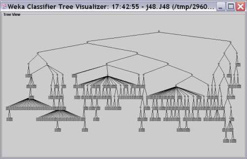
The details are:
 _corErr_50 <= 72: class1 (882.0/136.0)
 _corErr_50 > 72
 |   _corErr_50 <= 154
 |   |   _spec_2 = b
 |   |   |   _hiDist_13 = 0
 |   |   |   |   _corErr_11 <= 17: class1 (31.0/12.0)
 |   |   |   |   _corErr_11 > 17: class2 (19.0/2.0)
 |   |   |   _hiDist_13 = tr
 |   |   |   |   _corErr_31 <= 18: class1 (2.0)
 |   |   |   |   _corErr_31 > 18
 |   |   |   |   |   _inspEff_19 <= 33.742185: class1 (2.0)
 |   |   |   |   |   _inspEff_19 > 33.742185: class2 (56.0/6.0)
 |   |   _spec_2 = f
 |   |   |   _corErr_21 <= 22
 |   |   |   |   _detCap_38 <= 0.563188
 |   |   |   |   |   _inspDur_10 <= 117.043523
 |   |   |   |   |   |   _corErr_50 <= 120: class1 (11.0)
 |   |   |   |   |   |   _corErr_50 > 120
 |   |   |   |   |   |   |   _inspDur_40 <= 292.445892: class2 (8.0/1.0)
 |   |   |   |   |   |   |   _inspDur_40 > 292.445892: class1 (11.0/1.0)
 |   |   |   |   |   _inspDur_10 > 117.043523: class1 (19.0)
 |   |   |   |   _detCap_38 > 0.563188: class2 (6.0/1.0)
 |   |   |   _corErr_21 > 22: class2 (7.0/1.0)
 |   |   _spec_2 = n
 |   |   |   _inspEff_29 <= 336.924853: class2 (106.0/15.0)
 |   |   |   _inspEff_29 > 336.924853: class1 (5.0)
 |   |   _spec_2 = w
 |   |   |   _corErr_11 <= 3: class1 (2.0)
 |   |   |   _corErr_11 > 3
 |   |   |   |   _corErr_11 <= 4
 |   |   |   |   |   _inspEff_9 <= 32.423212: class2 (6.0)
 |   |   |   |   |   _inspEff_9 > 32.423212
 |   |   |   |   |   |   _inspDur_10 <= 35.939846
 |   |   |   |   |   |   |   _detCap_8 <= 0.110608: class2 (3.0/1.0)
 |   |   |   |   |   |   |   _detCap_8 > 0.110608: class1 (4.0)
 |   |   |   |   |   |   _inspDur_10 > 35.939846: class2 (4.0)
 |   |   |   |   _corErr_11 > 4
 |   |   |   |   |   _detCap_8 <= 0.145107
 |   |   |   |   |   |   _inspEff_9 <= 49.227938: class1 (8.0)
 |   |   |   |   |   |   _inspEff_9 > 49.227938
 |   |   |   |   |   |   |   _detCap_8 <= 0.131955: class2 (2.0)
 |   |   |   |   |   |   |   _detCap_8 > 0.131955: class1 (2.0)
 |   |   |   |   |   _detCap_8 > 0.145107
 |   |   |   |   |   |   _inspEff_9 <= 33.741217: class1 (10.0/3.0)
 |   |   |   |   |   |   _inspEff_9 > 33.741217: class2 (13.0/1.0)
 |   _corErr_50 > 154
 |   |   _detCap_8 <= 0.618237: class2 (73.0)
 |   |   _detCap_8 > 0.618237
 |   |   |   _inspDur_30 <= 137.500433: class3 (2.0)
 |   |   |   _inspDur_30 > 137.500433: class2 (6.0)
The learners are running but we haven't got much useful. Maybe treatment learning?
Using the techniques described at http://www.cs.pdx.edu/~timm/dm/rx.html. we find stable treatments:
 sirius$ tar3unix/bin/xval.sol tar3unix/bin/tar3.sol inspectd
 sirius$ stable XDFsum.out
 Freq   Lift Treatment
 ====   ==== =========
  10    2.25  _hidesignv2_15=[0.5]
  10    2.25  _hidesignv1_14=[0.3]
  10    2.25  _hidesign_12=[f]
   9    2.26  _hidesignv3_16=[0.7]
   5    2.27  _hidesign_12=[f] _inspDur_49=[2.6..4.7)
   4    2.38  _hidesign_12=[f] _hidesignv2_15=[0.5]
   4    2.35  _hidesignv1_14=[0.3] _loDist_23=[tr]
   4    2.34  _codev2_35=[0.5] _hiStaff_17=[4]
   4    2.32  _corErr_41=[72..105) _loStaff_27=[4]
   4    2.25  _hidesignv1_14=[0.3] _hidesignv3_16=[0.7]
   4    2.23  _hiStaff_17=[4] _hidesignv3_16=[0.7]
What is being said here is that there are three attribute settings that always resul in high lifts.
What does a lift of 2.35 look like? A manual inspection of TAR3's XDF files gives an example:
          class1:                                [     0%]
          class2:                                [     0%]
          class3:~~~~~~~                         [    20%]
          class4:~~~~~~~~~~~~~~~~~~~~~~~~~~~~~~  [    80%]
Recall the original distribution:
 class1| 519| **************************************** [ 40% ]
 class2| 260| ********************                     [ 20% ]
 class3| 260| ********************                     [ 20% ]
 class4| 260| ********************                     [ 20% ]
and the definitions of the classes.
 if utility < 9843 then class1
 else if utility < 10698 then class2
      else if utility < 11664 then class3
           else if utility < 14755 then class4
                else class5
Here's a little picture of the improvement:
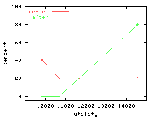
Generated by inspectlog.sh:
 cat<<-EOF>inspectlog.dat
        9853 40 0
        10698 20 0
        11664 20 20
        14555 20 80
 EOF
 cat<<-EOF>inspectlog.plt
 set yrange [-5:100]
 set key top left
 set ylabel "percent"
 set xrange [9000:15000]
 set xtics (10000,11000,12000,13000,14000)
 set xlabel "utility"
 set size 0.5,0.5
 set terminal png small color
 set output "inspectlog.png"
 plot "inspectlog.dat" using 1:2 title "before" with linesp,\
       "inspectlog.dat" using 1:3 title "after" with linesp
 EOF
 gnuplot inspectlog.plt
 chmod a+r inspectlog.png
The treatment learner is saying that the details of the inspection process (which on FFFF, FFFN,etc) is less important that other choices. How interesting.
 Tim Menzies ,
tim@menzies.us,
http://menzies.us
Tim Menzies ,
tim@menzies.us,
http://menzies.us
This page generated by Site:
see http://www.cs.pdx.edu/~timm/dm/site.html
 This site is built using PerlPod.
Style sheet switching method taken from Eddie Traversa's excellent and simple-to-apply tutorial: http://dhtmlnirvana.com/content/styleswitch/styleswitch1.html.
Search engine powered by ATOMZ http://www.atomz.com/search/. Note, the indexes to this site are only updated weekly (heh, its a free service- what more ja want?).
Icons on this site come from http://www.sql-news.de/rubriken/olap.asp and http://www.ifnet.it/webif/centrodi/eng/toolbar.htm.
The JAVA machine learners used at this site come from the extensive data mining libraries found in the University of Waikato's Environment for Knowledge Analysis (the WEKA) http://www.cs.waikato.ac.nz/ml/weka/
Copyright (C) Tim Menzies 2004
This program is free software; you can redistribute it and/or modify it under the terms of the GNU General Public License as published by the Free Software Foundation, version 2; see http://www.gnu.org/copyleft/gpl.html. This program is distributed in the hope that it will be useful, but WITHOUT ANY WARRANTY; without even the implied warranty of MERCHANTABILITY or FITNESS FOR A PARTICULAR PURPOSE. See the GNU General Public License for more details. You should have received a copy of the GNU General Public License along with this program; if not, write to the Free Software Foundation, Inc., 59 Temple Place - Suite 330, Boston, MA 02111-1307, USA.
The content from or through this web page are provided 'as is' and the author makes no warranties or representations regarding the accuracy or completeness of the information. Your use of this web page and information is at your own risk. You assume full responsibility and risk of loss resulting from the use of this web page or information. If your use of materials from this page results in the need for servicing, repair or correction of equipment, you assume any costs thereof. Follow all external links at your own risk and liability.