Inside Games

Steering

Think of a gang, patrolling at the front gate of a castle, protecting an area on a bridge.

Looking inside each members of the gang game, we may see

SteeringForce +=
    wander()            * wanderAmount        * wanderProirity +
    obstacleAvoidance() * avoidAmount         * avoidPriority +
    aligness()          * alignAmount         * alignPriority +
    cohesion()          * cohesionAmount      * cohesionPriority +
    seperation()        * seperationAmount    * seperationPriority +
    alignment()         * alignAmount         * alignPriority +
    wallAvoidance()     * wallAvoidanceAmount * wallAvoidPriority  +
    chasePrey()         * chaseAmount         * chasePriority +
    avoidPrey()         * avoidAmount         * avoidPriority 

What is going on here? A round robin between two models:

• A actor model: I think I want to steer here
• A physics model (walls, gravity, air or mud resistance): oh no you don't
  • E.g. flow fields

steer
  |
  |
  v
 Player ---> thrust

How to control a whole host of behaviors:.

Pattern Movements (Wandering)

When in doubt, pattern movement. At any "X", going in direction "Y", pick any neighbor at random, favoring those nearer your current compass bearing:

pattern[0]={1111111111
            1111111111
            1111111111
            1111111111
            1111111111
            1111111111
            1111111111}

pattern[1]={1...1..111
            .1.1..1...1
            1.1.......1
            .1..111.1.1
            1..1...1.1.
            1.1........
            11.........}

pattern[2]=

Bread crumbs

Actor X drops bread crumbs. Actor Y steers towards zones of higher bread crumb results.

Bread crumbing have some nice computational properties; e.g. very fast to compute.

Flocking

Kind of pattern movements, for groups.

Look around to a distance of "D" for an plus/minus "X" degrees from your current compass bearing:

• Increase "X" to make more of the flock spread wide, flock more together;
• Decrease "X" to turn the "flock" into a single file of actors, playing follow the leader.

With that knowledge, work out how much to operate, align, cohere:

	Separation: steer to avoid crowding local flock mates (give this one the highest priority)
	Alignment: steer towards the average heading of local flock mates
	Cohesion: steer to move toward the average position of local flock mates, maybe weighted by your compass bearing 741 973 741

(See also Lennard-Jones functions for combining the above into one equation.)

Leader Following

Do a weighted sum of the neighborhood, giving a "leader" more weight than the rest of the flock.

Now the problem of programming the flock reduces to just the problem of programming the leader.

Note: the leader can be selected dynamically:

• E.g. you want to herd the flock through a gate;
• The "leader" is the flock member closest to the gate;
• So, if the leader falls, you can automatically pick another another leader

Predation

Predict where the food will be, steer towards there.

Prey avoidance

Predict where the prey will be, steer away from there.

Or, with knowledge of the terrain, find a predator's blind spot (behind a rock) and go steer to there.

Obstacle avoidance

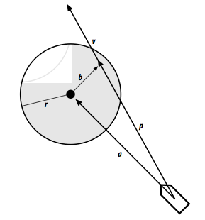
Extend "feelers".

If they fall within "r" of some obstacle, then insert a steering force "b" to deflect the actor

Path finding and way points

Given a terrain map of regions (rooms, valleys with passes between them, oceans connected by straights),

• Reduce the navigation problem to paths between way points.

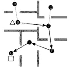
To compute way points:

• Place points in every room/region of the terrain map
• Jiggle them so they they are in line of sight of the most number of other points (minimum of one)
• Pre-computer and cache nearest adjacent nodes
• Store the adjacency matrix M1[u,v] means path from u to v

  M1=    A B C D E F G
       A . 1 . . . . .
       B . . 1 . . . .
       C . . . 1 1 . .
       D . . . . . . .
       E . . . . . 1 .
       F . . . . . . 1
       G . . . . . . .
  

• Complete the matrix. If paths bi-directional, then If M2[u,v] = M1[u,v] or M1[v,u]

  M2=    A B C D E F G
       A . 1 . . . . .
       B 1 . 1 . . . .
       C . 1 . 1 1 . .
       D . . 1 . . . .
       E . . 1 . . 1 .
       F . . . . 1 . 1
       G . . . . . 1 .
  

• Note that:
  • M stores all paths of length one.
  • M² stores all paths of length two.
  • M³ stores all paths of length three.
  • M^* (transitive closure) stores all paths of all lengths (see any algorithms book)
    • Loop detection: transitive closure for N vertices O(N³). Loop if "u" is in its own transitive closure.

If you want some geography, add distance measure instead of just "1"

D1=    A B C D E F G
     A . 4 . . . . .
     B . . 2 . . . .
     C . . . 9 7 . .
     D . . . . . . .
     E . . . . . 8 .
     F . . . . . . 3
     G . . . . . . .

These numbers can reflect difficulty in traversing some region (e.g. mud, quicksand, steep slopes)

Navigation in two steps: go straight to the nearest way point, then path follow from weigh point to weigh point.

• "u := extract_min(Q)" searches for the vertex u in the vertex set Q that has the least dist[u] value.
• (And as a side-effect, "u"" is removed from "Q")
• "length(u, v) = D[u,v]
• Built a shortest path tree between all way points

   1  function Dijkstra(Graph, source):
   2      for each vertex v in Graph:           // Initializations
   3          dist[v] := infinity               // Unknown distance function from source to v
   4          previous[v] := undefined
   5      dist[source] := 0                     // Distance from source to source
   6      Q := copy(Graph)                      // All nodes in the graph are unoptimized - thus are in Q
   7      while Q is not empty:                 // The main loop
   8          u := extract_min(Q)               // Remove and return best vertex from nodes in two given nodes
                                                // we would use a path finding algorithm on the new graph, such as depth-first search.
   9          for each neighbor v of u:         // where v has not yet been removed from Q.
  10              alt = dist[u] + length(u, v)
  11              if alt < dist[v]              // Relax (u,v)
  12                  dist[v] := alt
  13                  previous[v] := u
  14      return previous[]
  

When wondering a path, remember to stagger a little and steer more at corners.

And for crowds to walk paths, add obstacle avoidance.

Influence Maps

Recall our geography maps:

D1=    A B C D E F G
     A . 4 . . . . .
     B . . 2 . . . .
     C . . . 9 7 . .
     D . . . . . . .
     E . . . . . 8 .
     F . . . . . . 3
     G . . . . . . .

Remember that these numbers can reflect difficulty in traversing some region (e.g. mud, quicksand, steep slopes)

An influence map is a second "geography" map that changes at runtime. E.g. suppose you keep dying every time you walk from G to A:

Inf=    A B C D E F G
     A . . . . . . .
     B . . . . . . .
     C . . . . . . .
     D . . . . . . .
     E . . . . . . .
     F . . . . . . .
     G 10 . . . . . .

So now we can do A* to minimize g(x)+h(x) where "h=D+Inf"

Two-player Systems

So if the above methods are all standard, the enemy knows them too.

Q1: How can you reason about the enemy reasoning about your reasoning?

• A1: MinMax trees

Q2: How you do the above faster?

• A2: Alpha-Beta pruning. Each node is shown with the [min,max] range. In general the [min,max] bounds become tighter and tighter as you proceed down the tree from the root. Sometimes, you can skip a subtree if its min/max is out-of-bounds of the current min-max.

See http://www.ocf.berkeley.edu/~yosenl/extras/alphabeta/alphabeta.html

There is a common illusion that we first generate a n-ply minmax tree and then apply alpha-beta prune. No, we generate the tree and apply alpha-beta prune at the same time (otherwise, no point).

How effective is alpha-beta pruning? It depends on the order in which children are visited. If children of a node are visited in the worst possible order, it may be that no pruning occurs. For max nodes, we want to visit the best child first so that time is not wasted in the rest of the children exploring worse scenarios. For min nodes, we want to visit the worst child first (from our perspective, not the opponent's.) There are two obvious sources of this information:

• A static evaluator function can be used to rank the child nodes
• Previous searches of the game tree (for example, from previous moves) performed minimax evaluations of many game positions. If available, these values may be used to rank the nodes.

When the optimal child is selected at every opportunity, alpha-beta pruning causes all the rest of the children to be pruned away at every other level of the tree; only that one child is explored. This means that on average the tree can searched twice as deeply as before?a huge increase in searching performance.