Search

Search is a universal problem solving mechanism in AI. The sequence of steps required to solve a problem is not known a priori and it must be determined by a search exploration of alternatives.

In computer science, a state space is a description of a configuration of discrete states used as a simple model of machines. Formally, it can be defined as a tuple [N, A, S, G] where:

• S is a nonempty subset of N that contains start states
• G is a nonempty subset of N that contains the goal states.
• N is a set of states, each with "successors"
• A is a set of arcs connecting each state to its successors

Often, there are oracles that offer clues on the current progress in the search

• g(x) is a measure of "distance" of state "x" from start.
• h(x) is a measure of "cost" required to get from state "x" to the goal.

While "g(x)" can be known exactly (since it is a log of the past) while "h(x)" is a heuristic guess-timate (since we have not searched there yet).

The state space is what state space search searches in. Graph theory is helpful in understanding and reasoning about state spaces.

A state space has some common properties:

• complexity, where branching factor "b" is important
• structure of the space, see also graph theory:
  • directionality of arcs
  • tree
  • rooted graph

In this lecture, we will explore two kinds of search engines:

• Ordered-search; e.g. the tree and graph searchers discussed below. In this kind of search, the solutions spreads out in a wave over over some solution space.
• Unordered-search where a partial solution is quickly (?randomly) generated, then maybe fiddled with. A common unordered search method is to generate a number of slots, each with random values as done in simulated annealing or MAXWALKSAT (discussed below).

Ordered search is useful for problems with some inherent ordering (e.g.) walking a maze.

Unordered search is useful for problems where ordering does not matter. For example, if a simulator accepts N inputs, then an unordered search might supply M ≤ N inputs and the rest are filled in at random.

Problem Search Strategies

In practice, S may not be pre-computed and cached. Rather, the successors to some state "s" may be computed using some "successors" function only when, or if, we ever reach "s". In the following code:

• Some "goal-p" function checks if we have arrived at our goal.
• Some "combiner" function joins the successors with the rest of the states (maybe removing duplicates).

(defun tree-search (states goal-p  successors combiner)
  (labels ((next  ()       (funcall successors (first states)))
           (more-states () (funcall combiner   (next) (rest states))

   (cond ((null states) nil)                              ; failure. boo!
         ((funcall goal-p (first states)) (first states)) ; success!
         (t  (tree-search                                 ; more to do
               (more-states) goal-p successors combiner))))

• Devise a representation scheme for states
• Describe an initial and a final state
• Describe operators
• Select which state to expand next
• Recognize the goal when generated

Example: Monkey pushing a chair under a banana, climbs the chair, eats the banana

(defparameter *banana-ops*
  (list
    (op 'climb-on-chair
        :preconds '(chair-at-middle-room at-middle-room on-floor)
        :add-list '(at-bananas on-chair)
        :del-list '(at-middle-room on-floor))
    (op 'push-chair-from-door-to-middle-room
        :preconds '(chair-at-door at-door)
        :add-list '(chair-at-middle-room at-middle-room)
        :del-list '(chair-at-door at-door))
    (op 'walk-from-door-to-middle-room
        :preconds '(at-door on-floor)
        :add-list '(at-middle-room)
        :del-list '(at-door))
    (op 'grasp-bananas
        :preconds '(at-bananas empty-handed)
        :add-list '(has-bananas)
        :del-list '(empty-handed))
    (op 'drop-ball
        :preconds '(has-ball)
        :add-list '(empty-handed)
        :del-list '(has-ball))
    (op 'eat-bananas
        :preconds '(has-bananas)
        :add-list '(empty-handed not-hungry)
        :del-list '(has-bananas hungry))))

If the search space is small, then it is possible to write it manually (see above).

More commonly, the search space is auto-generated from some other representations (like the two examples that follow).

Here's walking a maze where "op" is inferred from the maze description:

(defparameter *maze-ops*
  (mappend #'make-maze-ops
     '((1 2) (2 3) (3 4) (4 9) (9 14) (9 8) (8 7) (7 12) (12 13)
       (12 11) (11 6) (11 16) (16 17) (17 22) (21 22) (22 23)
       (23 18) (23 24) (24 19) (19 20) (20 15) (15 10) (10 5) (20 25))))

(defun make-maze-op (here there)
  "Make an operator to move between two places"
  (op `(move from ,here to ,there)
      :preconds `((at ,here))
      :add-list `((at ,there))
      :del-list `((at ,here))))

(defun make-maze-ops (pair)
  "Make maze ops in both directions"
  (list (make-maze-op (first pair) (second pair))
        (make-maze-op (second pair) (first pair))))

(defun move-op (a b c)
  "Make an operator to move A from B to C."
  (op `(move ,a from ,b to ,c)
      :preconds `((space on ,a) (space on ,c) (,a on ,b))
      :add-list (move-ons a b c)
      :del-list (move-ons a c b)))

(defun move-ons (a b c)
  (if (eq b 'table)
      `((,a on ,c))
      `((,a on ,c) (space on ,b))))

(defun make-block-ops (blocks)
  (let ((ops nil))
    (dolist (a blocks)
      (dolist (b blocks)
        (unless (equal a b)
          (dolist (c blocks)
            (unless (or (equal c a) (equal c b))
              (push (move-op a b c) ops)))
          (push (move-op a 'table b) ops)
          (push (move-op a b 'table) ops))))
    ops))

Search Trees

General search methods to:

• Explore to depth "d"
• A tree that branches at a rate of "b" out-arcs per node

• running time O(b^d)
• least space: O(b * d)
  • At most, one branch from root to a leaf, knowing that there are "b" options per node.
    • may not find the minimum cost solution

• running time O(b^d)
• most space: space requirements O(b^d)
• least cost: (shortest path to the goal)
• Variants: Given that you've reached depth "d", score the current partial solutions.
  • best-first search
    • Sort the solutions and expand them in the order best to worst.
  • beam-search
    • Only expand the "N" best ones
    • Keep N small (10 or 20) to constrain search size.
    • Note: small beams mean less memory but make the search incomplete (may miss solutions).

• Depth search to maximum depth Max
• Repeat for Max+1
• running time O(b^d)
• space requirements O(b*d)
• finds the minimum cost solution (shortest path to the goal)
• It can be shown that this algorithm visits all nodes at most

  M(b,d) <= b^d*(1 - 1/b)^(-2)
  

  As the branching factor increases, the extra overhead of DFID's repeated search over breadth-first "b^d" search approaches unity:
  • When b=2, M(b,d) ≤ 4 * b^d
  • When b=3, M(b,d) ≤ 9/4 * b^d
  • When b=4, M(b,d) ≤ 16/9 * b^d
  • When b=5, M(b,d) ≤ 25/16 * b^d
• Same iterative widening methods can be applied to any search

• add a "precursors" function that returns parents of the current state (i.e. the opposite to "successors").
• Run two searches (forwards and backwards) it they ever meet, stop

For source code on the above, see here.

Stochastic Tree Search

• Start at "start".
• If too many restarts, stop.
• Take any successor.
• Repeat till you hit a dead-end or "goal".
• If dead-end, then restart

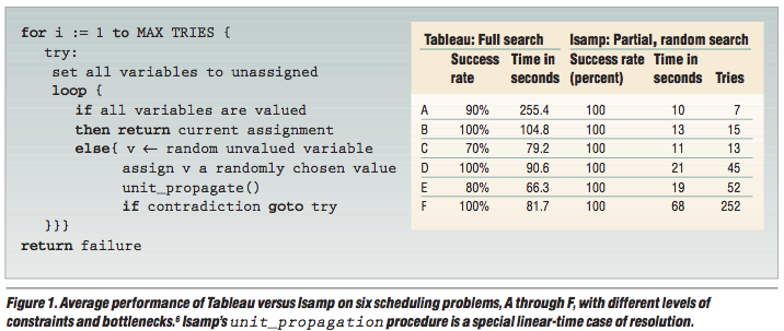
This stochastic tree search can be readily adapted to other problem types.

Eg#1: scheduling problems

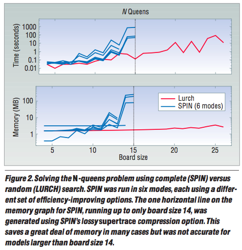
Eg#2: N-queens with the lurch algorithm. From state "x", pick an out-arc at random. Follow it to some max depth. Restart.

Q: Why does Isamp work so well. work so well?

• A: Few solutions, large space between them. Complete search wastes a lot of time if it lucks into a poor initial set of choices.
• See also stochastic search, below.

Graph search

Like tree search, but with a *visited* list that checks if some state has not been reached before.

Visited list can take a lot of memory

• Standard fix: some hashing scheme so that states get stored in a compact representation
• Incomplete: if different reached states happen to hash to the same value.

A* search: standard game playing technique:

• Best-first search of graph with a *visited* list where states are sorted by "g+h"
• g(x)= Cost to reach state "x" from start
• h(x)= Heuristic estimate of cost to go from "x" to goal
• Important: h(x) must under-estimate cost from "x" to goal
  • E.g. straight line "as the bird flies" distance to shop at the Target store is less than the actual driving distance
  • Assuming under-estimates, then A* is optimal.
    • Let f(x)=g(x)+h(x).
    • Compare two solutions s1, s2 that go from "x" to goal.
    • actual > f(s1) due to the under-estimation assumption
    • And, at termination (by definition) f(s1) < f(s2)
    • So actual > f(s2) > f(s1) ; i.e. using s1 was optional
    If g(x) over-estimates then
    • actual ≤ f(s1)
    • At termination, other, worse solution "s2" has f(s1) < f(s2) (as before).
    • But we don't know if s2 is between s1 and actual.

Unordered searchers

Strangely, order may not matter. Rather than struggle with lots of tricky decisions,

• exploit speed of modern CPUs, CPU farms.
• try lots of possibilities, very quickly

• current := a random solution across the space
• If its better than anything seen so far, then best := current

• Change part of the current solution at random

• Change that part of the solution that most improves score

Simulated Annealing

S. Kirkpatrick and C. D. Gelatt and M. P. Vecchi Optimization by Simulated Annealing, Science, Number 4598, 13 May 1983, volume 220, 4598, pages 671680,1983.

s := s0; e := E(s)                     // Initial state, energy.
sb := s; eb := e                       // Initial "best" solution
k := 0                                 // Energy evaluation count.
WHILE k < kmax and e > emax            // While time remains & not good enough:
  sn := neighbor(s)                   //   Pick some neighbor.
  en := E(sn)                          //   Compute its energy.
  IF    en < eb                        //   Is this a new best?
  THEN  sb := sn; eb := en             //     Yes, save it.
  FI
  IF random() > P(e, en, k/kmax)       //   Should we move to it?
  THEN  s := sn; e := en               //     Yes, change state.
  FI
  k := k + 1                           //   One more evaluation done                        
RETURN sb                              // Return the best solution found.

Note the space requirements for SA: only enough RAM to hold 3 solutions. Very good for old fashioned machines.

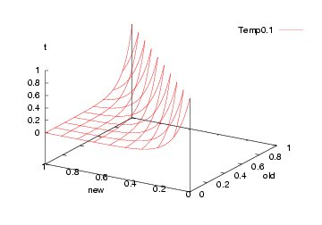
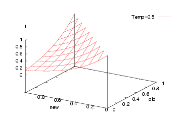
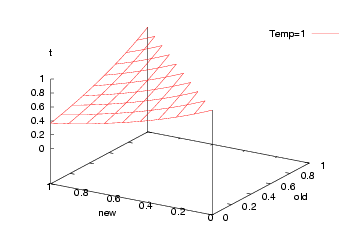
But what to us for the probability function "P"? This is standard function:

FUNCTION P(old,new,t) = e^((old-new)/t)

• Initially:
• Subsequently:
• Finally:

That is, we jump to a worse solution when "random() > P" in two cases:

• The sensible case: if "new" is greater than "old"
• The crazy case: earlier in the run (when "t" is small)

Note that such crazy jumps let us escape local minima.

MAXWALKSAT

Kautz, H., Selman, B., & Jiang, Y. A general stochastic approach to solving problems with hard and soft constraints. In D. Gu, J. Du and P. Pardalos (Eds.), The satisfiability problem: Theory and applications, 573586. New York, NY, 1997.

State of the art search algorithm.

FOR i = 1 to max-tries DO
  solution = random assignment  
  FOR j =1 to max-changes DO
    IF    score(solution) > threshold
    THEN  RETURN solution
    FI
    c = random part of solution 
    IF    p < random()
    THEN  change a random setting in c
    ELSE  change setting in c that maximizes score(solution) 
    FI
RETURN failure, best solution found

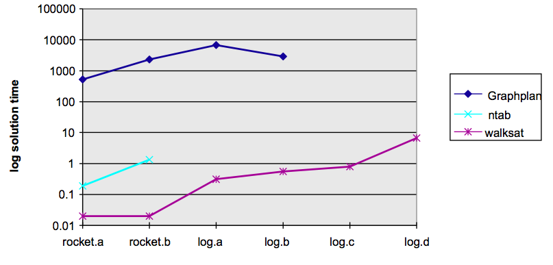
This is a very successful algorithm. Here's some performance of WALKSAT (a simpler version of MAXWALKSAT) against a complete search

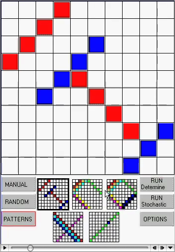
You saw another example in the introduction to this subject. The movie at right shows two AI algorithms t$ solve the "latin's square" problem: i.e. pick an initial pattern, then try to fill in the rest of the square with no two colors on the same row or column.

• The deterministic method is the kind of exhaustive theorem proving method used in the 1960s and 1970s that convinced people that "AI can never work".
• The stochastic method is a 1990s-style AI algorithm that makes some initial guess, then refines that guess based on logic feedback.

This stochastic local search kills the latin squares problem (and, incidently, many other problems).