» fss
Feature Subset Selection (FSS)
- Occam's Razor - The English philosopher, William of Occam
(1300-1349) propounded Occam's Razor:
- Entia non sunt multiplicanda praeter necessitatem.
- (Latin for "Entities should not be multiplied more than necessary"). That is, the fewer assumptions an explanation of a phenomenon depends on, the better it is.
- (BTW, Occam's razor did not survive into the 21st
century.
- The data mining community modified it to the Minimum Description Length (MDL) principle.
- MDL: the best theory is the smallest BOTH is size AND number of errors).
The case for FSS
Repeated result: throwing out features rarely damages a theory

Feature removal enables the processing of very large data sets (e.g. see the text mining example, below).
And, finally, feature removal is sometimes very useful:
- E.g. linear regression on
bn.arff yielded:
Defects = 82.2602 * S1=L,M,VH + 158.6082 * S1=M,VH + 249.407 * S1=VH + 41.0281 * S2=L,H + 68.9153 * S2=H + 151.9207 * S3=M,H + 125.4786 * S3=H + 257.8698 * S4=H,M,VL + 108.1679 * S4=VL + 134.9064 * S5=L,M + -385.7142 * S6=H,M,VH + 115.5933 * S6=VH + -178.9595 * S7=H,L,M,VL + ... [ 50 lines deleted ] - On a 10-way cross-validation, this correlates 0.45 from predicted to actuals.
- 10 times, take 90% of the date and run a
WRAPPER- a best first search through combinations of
attributes. At each step, linear regression was called to
asses a particular combination of attributes. In those ten
experiments, WRAPPER found that adding feature X to features
A,B,C,... improved correlation the following number of times:
number of folds (%) attribute 2( 20 %) 1 S1 0( 0 %) 2 S2 2( 20 %) 3 S3 1( 10 %) 4 S4 0( 0 %) 5 S5 1( 10 %) 6 S6 6( 60 %) 7 S7 <== 1( 10 %) 8 F1 1( 10 %) 9 F2 2( 20 %) 10 F3 2( 20 %) 11 D1 0( 0 %) 12 D2 5( 50 %) 13 D3 <== 0( 0 %) 14 D4 0( 0 %) 15 T1 1( 10 %) 16 T2 1( 10 %) 17 T3 1( 10 %) 18 T4 0( 0 %) 19 P1 1( 10 %) 20 P2 0( 0 %) 21 P3 1( 10 %) 22 P4 6( 60 %) 23 P5 <== 1( 10 %) 24 P6 2( 20 %) 25 P7 1( 10 %) 26 P8 0( 0 %) 27 P9 2( 20 %) 28 Hours 8( 80 %) 29 KLoC <== 4( 40 %) 30 Language 3( 30 %) 32 log(hours) - Four variables appeared in the majority of folds. A
second run did a 10-way using just those variables to yield a
smaller model with (much) larger correlation (98\%):
Defects =
    876.3379 * S7=VL +
   -292.9474 * D3=L,M +
    483.6206 * P5=M +
      5.5113 * KLoC +
     95.4278
Excess attributes
- Confuse decision tree learners
- Too much early splitting of data
- Less data available for each sub-tree
- Too many things correlated to class?
- Dump some of them!
Why FSS?
- throw away noisy attributes
- throw away redundant attributes
- smaller model= better accuracies (often)
- smaller model= simpler explanation
- smaller model= less variance
- smaller model= any downstream processing will thank you
Problem
- Exploring all subsets exponential
- Need heuristic methods to cull search;
- e.g. forward/back select
-
Forward select:
- start with empty set
- grow via hill climbing:
- repeat
- try adding one thing and if that improves things
- try again using the remaining attributes
- until no improvement after N additions OR nothing to add
-
Back select
- as above but start with all attributes and discard, don't add
-
Usually, we throw away most attributes:
- so forward select often better
- exception: J48 exploits interactions more than,say, NB.
- so, possibly, back select is better when wrapping j48
- so, possibly, forward select is as good as it gets for NB
FSS types:


-
filters vs wrappers:
- wrappers: use an actual target learners e.g. WRAPPER
- filters: study aspects of the data e.g. the rest
- filters are faster!
- wrappers exploit bias of target learner so often
perform better, when they terminate
- don't terminate on large data sets
-
solo vs combinations:
- evaluate solo attributes: e.g. Tf*IDF, LOR, INFO GAIN, RELIEF
- evaluate combinations: e.g. PCA, SVD, CFS, CBS, WRAPPER
- solos can be faster than combinations
-
supervised vs unsupervised:
- use/ignores class values e.g. PCA/SVD is unsupervised, reset supervised
-
numeric vs discrete search methods
-
ranker: for schemes that numerically score attributes e.g. RELIEF, INFO GAIN,
-
best first: for schemes that do heuristic search e.g. CBS, CFS, WRAPPER
-
INFO GAIN
- often useful in high-dimensional problems (since, like
Tf*IDF) it runs in linear time.
- real simple to calculate
- attributes scored based on info gain: H(C) - H(C|A): see lecture on decision tree learning.
- Sort of like doing decision tree learning, just to one level.
RELIEF
- Kononenko97
- useful attributes differentiate between instances from other class
- randomly pick some instances (here, 250)
- find something similar, in an another class
- compute distance this one to the other one
- Stochastic sampler: scales to large data sets.
- Binary RELIEF (two class system) for "n" instances for
weights on features "F"
set all weights W[f]=0 for i = 1 to n; do randomly select instance R with class C find nearest hit H // closest thing of same class find nearest miss M // closest thing of difference class for f = 1 to #features; do W[f] = W[f] - diff(f,R,H)/n + diff(f,R,M)/n done done - diff:
- discrete differences: 0 if same 1 if not.
- continuous: differences absolute differences
- normalized to 0:1
- When values are missing, see Kononenko97, p4.
- N-class RELIEF: not 1 near hit/miss, but k nearest misses
for each class C
W[f]= W[f] - ∑i=1..k diff(f,R, Hi) / (n*k)
           + ∑C &ne class(R) ∑i=1..k (
                                P(C) / ( 1 - P(class(R)))
                                * diff(f,R, Mi(C)) / (n*k)
                               )
The P(C) / (1 - P(class(R)) expression is a normalization function that- demotes the effect of R from rare classes
- and rewards the effect of near hits from common classes.
CBS (consistency-based evaluation)
- Seek combinations of attributes that divide data
containing a strong single class majority.
- Kind of like info gain, but emphasis of single winner
- Discrete attributes
- Forward select to find subsets of attributes
WRAPPER
- Forward select attributes
- score each combination using a 5-way cross val
- When wrapping, best to try different target learners
- Check that we aren't over exploiting the learner's bias
- e.g. J48 and NB

PRINCIPAL COMPONENTS ANALYSIS (PCA)
(The traditional way to do FSS.)
- Only unsupervised method studied here
- Transform dimensions
- Find covariance matrix C[i,j] is the correlation i to j;
- C[i,i]=1;
- C[i,j]=C[j,i]
- Find eigenvectors
- Transform the original space to the eigenvectors
- Rank them by the variance in their predictions
- Report the top ranked vectors

-
Makes things easier, right? Well...
if   domain1  <= 0.180
then NoDefects
else if domain1 > 0.180
     then if domain1 <= 0.371 then NoDefects
     else if domain1 > 0.371 then Defects


domain1 = 0.241 * loc     + 0.236 * v(g)
        + 0.222 * ev(g)   + 0.236 * iv(g)     + 0.241 *  n
        + 0.238 * v       - 0.086 * l         + 0.199  * d
        + 0.216 * i       + 0.225 * e + 0.236 * b + 0.221  * t
        + 0.241 * lOCode  + 0.179 * lOComment
        + 0.221 * lOBlank + 0.158 * lOCodeAndComment
        + 0.163 * uniqO p + 0.234 * uniqOpnd
        + 0.241 * totalOp + 0.241 * totalOpnd
        + 0.236 * branchCount
Latent Semantic Indexing
-
Performing PCA is the equivalent of performing Singular Value Decomposition (SVD) on the data.
-
Any n * m matrix X (of terms n in documents m) can be rewritten as:
- X = To * So * Do'
- So is a diagonal matrix scoring attributes, top to bottom, most interesting to least interesting
- We can shrink X by dumping the duller (lower) rows of So

- Latent Semantic Indexing is a method for selecting informative subspaces of feature spaces.
- It was developed for information retrieval to reveal semantic information from document co-occurrences.
- Terms that did not appear in a document may still associate with a document.
-
LSI derives uncorrelated index factors that might be considered artificial concepts.
-
SVD easy to perform in Matlab
- Also, there is some C-code.
- Also Java Classes
available
- class SingularValueDecomposition
- Constructor: SingularValueDecomposition(Matrix Arg)
- Methods: GetS(); GetU(); GetV(); (U,V correspond to T,D)
- class SingularValueDecomposition
- Be careful about using these tools blindly
- It is no harm to understand what is going on!
-
The Matrix Cookbook
-
Note: major win for SVD/LSI: scales very well.
- Research possibility: text mining for software
engineering
- typically very small corpuses
- so might we find better FSS for text mining than SVD/LSI
- Research possibility: text mining for software
engineering
CFS (correlation-based feature selection)
- Scores high subsets with strong correlation to class and weak correlation to each other.
- Numerator: how predictive
- Denominator: how redundant
- FIRST ranks correlation of solo attributes
- THEN heuristic search to explore subsets
And the winner is:
- Wrapper! and it that is too slow...
- CFS, Relief are best all round performers
- CFS selects fewer features
- Phew. Hall invented CFS
Other Methods
Other methods not explored by Hall and Holmes...
- Note: the text mining literature has yet to make such an assessment. Usually, SVD rules. But see An Approach to Classify Software Maintenance Requests, from ICSM 2002, for a nice comparison of nearest neighbor, CART, Bayes classifiers, and some other information retrieval methods).
-
Using random forests for feature selection of the mth variable:
- randomly permute all values of the mth variable in the oob data
- Put these altered oob x-values down the tree and get classifications.
- Proceed as though computing a new internal error rate (i.e. run the classifier).
- The amount by which this new error exceeds the original test set error is defined as the importance of the mth variable.
FastMap
When data to large for LDA,PCA then use Fastmap.
To map N points in D dimensions to D-1:
- Pick any point
- In N comparisons, find the left point furthest away from that point.
- In N comparisons, find the right point furthest away from left
- Draw a line from left to right
- Draw a plane orthogonal to that line;
- Project all the points onto that line using the
cosine rule: see the FastMap paper for the details.
- Its kinda like you shine a light on the points and mark their positions on the plane.
- Throw away the line and keep the projection of the points on the plane.
To map down N points in D dimensions down to D=3 (so you can visualize it); repeat the above process D-3 times.
Heuristic: does not do as well as (say) PCA.
- But runs fast
- Scales (2N comparisons, not N2 at each step)
- Does not do much worse than PCA.
IMPORTANT NOTE: PCA, LSI, FastMap, etc ...:
- Do not reduce the number of attributes. Rather they combine the existing attributes into a smaller number of synthesized attributes.
- Are unsupervised methods since they do not use the class variable to control their synthesis.
Tf*IDF
FSS is essential in text mining:
- Consider a matrix of 1000 documents (in the rows)
- Each column is one unique word used in those documents.
- Such a matrix will be wide (10,000s to 100,000s of columns)...
- And quite sparse (most words appear in very few documents).
Before doing anything else, remove all the words you can.
To begin with:
- Send all to lower case;
- remove stop words (boring words like "a above above..") see examples at http://www.dcs.gla.ac.uk/idom/irresources/linguisticutils/stop_words> (Warning: don't remove words that are important to your domain.)
- Apply stemming: These words are all "connect": connect, connected, connecting, connection,connections. Can be unified using (e.g.) PorterStemming?: the standard stemming algorithm, available in multiple languages: http://www.tartarus.org/~martin/PorterStemmer/ (see also: Porter's definition of the algorithm
- Reject all but the top k most interesting words
But what makes a word interesting:
- Interesting if frequent OR usually appears in just a few paragraphs
- TF*IDF (term frequency, inverse document frequency)
- Interesting =
-
F(i,j) * log((Number of documents)/(number of documents including word i))
- F(i,j): frequency of word i in document j
- Often, on a very small percentage of the words are high scorers, so a common transform is to just use the high fliers. e.g. here's data from five bug tracking systems a,b,c,d,e:

Build a symbol table of all the remaining words
- Convert strings to pointers into the symbol table
- So "the cat sat on the cat" becomes 6 pointers to 4 words
IMPORTANT: all the above a linear-time transforms requiring three passes (at most) over the data. For text mining, such efficiency is vital.
Note: At ICSM'08, Menzies and Marcus reduced 10,000 words to the top 100 Tf*IDF terms, then sorted those by InfoGain.
- Rules were learned using the top 100, 50,25,12,6,3 terms (as sorted by InfoGain)
- Rules from top 3 terms worked nearly as well as rules learned from top 100 terms.
- Perhaps there is more structure that we would like to think in "unstructured" natural language.
Nomograms
[Mozina04] argue that what really matters is the effect of a cell on the output variables. With knowledge of this goal, it is possible to design a visualization, called a nomogram, of that data. Nomograms do not confuse the user with needless detail. For example, here's nomogram describing who survived and who died on the Titanic:

Of 2201 passengers on Titanic, 711 (32.3%) survived. To predict who will survive, the contribution of each attribute is measured as a point score (topmost axis in the nomogram), and the individual point scores are summed to determine the probability of survival (bottom two axes of the nomogram).
The nomogram shows the case when we know that the passenger is a child; this score is slightly less than 50 points, and increases the posterior probability to about 52%. If we further know that the child traveled in first class (about 70 points), the points would sum to about 120, with a corresponding probability of survival of about 80%.
It is simple to calculate nomogram values for single ranges. All we want is something that is far more probable in a goal class than in other classes.
- Suppose there is a class you like C and a bunch of others you hate.
- Let the bad classes be combined together into a group we'll call notC
- Let the frequencies of C and notC be N1 and N2.
- Let an attribute range appears with frequency F1 and F2 in C1 and notC.
- Then the log(OR) = log ( (N1 / H1) / (N2 / H2) )
We use logs since products can be visualized via simple addition. This addition can be converted back to a probability as follows. If the sum is "f" and the target class occurs "N" times out of "I" instances, then the probability of that class is "p=N/I" and and the sum's probability is:
function points2p(f,p) { return 1 / (1 + E^(-1*log(p/(1 - p)) - f )) }
(For the derivation of this expression, see equation 7 of
[Mozina04].
Note that their equation has a one-bracket typo.)
Besides enabling prediction, the nomogram reveals the structure of the model and the relative influences of attribute values on the chances of surviving. For the Titanic data set:
- Gender is an attribute with the biggest potential influence on the probability of survival: being female increases the chances of survival the most (100 points), while being male decreases it (about 30 points). The corresponding line in the nomogram for this attribute is the longest.
- Age is apparently the least influential, where being a child increases the probability of survival.
- Most lucky were also the passengers of the first class for which, considering the status only, the probability of survival was much higher than the prior.
Therefore, with nomograms, we can play cost-benefit games. Consider the survival benefits of
- sex=female (72%)
- sex=female and class=first (92%)
- sex=female and class=first and age=child (95%)
Note that pretending to be a child has much less benefit than the other two steps. This is important since the more elaborate the model, the more demanding it becomes. Simpler models are faster to apply, use less resources (sensors and actuators), etc. So when the iceberg hits, get into a dress and buy a first-class ticket. But forget the lollipop.
I've applied some nomogram visualization to the output of Fenton's Bayes nets. The results found some simple rules that predicted for worst case defects:

B-squared
We've had some problems with nomograms where something is relatively more common in one class than other but, in absolute terms, is still rare.
E.g. in 10,000 examples, if Martians appear twice as much in the low IQ sample than the high IQ sample, then nomograms would say that being from Mars predicts for being dumb.
But the number of Martians on Earth is very small (100, or even less) so compared to the size of the total population, this is not an interesting finding.
Hence, we've modified Nomograms as follows.
- First, we use Bayes theorem to find the probability that a range is in the goal class rather than in the others.
- Then we multiply that probability by the frequency with which that range appears in the desired class.
- Mathematically, this is just:
- Suppose there is a class you like C and a bunch of others you hate.
- Let the bad classes be combined together into a group we'll call notC
- Let the frequencies of C and notC be N1 and N2.
- Let two attribute range X appears with frequency F1 and F2 in C1 and notC.
- Then let "b" (for best) be F1/N1
- Then let "r" (for rest) be F2/N2
- Then let the prob(C|X) = b/(b+r)
- And let's set the score of each range to be
- zero if r is less than b
- or, otherwise, b^2/(b+r).
The squared "b" value penalizes any X that occurs with a low frequency in C.
We can generate the same nomogram graphs, as above, using B-squared instead of LOR.
Beyond Feature Selection
Note that the LOR and B-squared are range selectors, not feature feature selectors. That is, they don't just comment on which attributes are important, but which ranges within those attributes are important.
This means we can use "feature selection" for other applications.
Instance Selection
Just as it it useful to prune features (columns), it is also useful to either prune instances (rows) or replace a larger number of rows with a smaller number of artificially generated representative examples.
- Some rows are outliers from bad data collection and should be removed.
- Any visualization, explanation, clustering system is optimized by pruning away spurious information.
- Removing some (most) of the rows usually does not degrade performance Chang's instance selector replaced training sets of size rows1 = (514, 150, 66) with reduced sets of of size rows2 = (34, 14, 6) (respectively), with no performance degradation. Note that rows2 contains only (7, 9, 9)% of the original data. (Chang, "Finding prototypes for nearest neighbor classifiers", IEEE Trans. on Computers, pp. 1179-1185, 1974).
- Removing rows can make some inference more robust:
- Consider classification using nearest neighbors.
- After instance selection, the neighbors are further away.
- Hence, any errors in measurements on the test instance are {\em less} likely to cause a change in classification.
How to perform instance selection?
- The slow way (O(N2)): pair all rows with their nearest neighbor, find the median of each pair, synthesize new instance at that location. Repeat, pairing the pairs etc to form a tree binary whose leaves are real instances and whose internal nodes are artificially created node. To generate N instances that represent the original data, descend log2 into the tree.
- The fast way (O(N)): find the topped ranked ranges (using Nomograms or B-squared) and remove all rows that have less than X of those top ranges.
Rule Generation
A rule condition is a collection of ranges, combined as disjuncts, conjuncts, negation.
If we have a range selector, why not run it as a pre-processor to a rule generator?
A Better PRISM
- while some instances of that class remain
-
- find one rule that covers most instances of one class
- Print that rule;
- remove instances that are covered (i.e. match) the rule

Possible rule set for class b:
- If x 1.2 then class = b
- If x > 1.2 and y 2.6 then class = b
- More rules could be added for perfect rule set
The PRISM Algorithm
A simple covering algorithm developed by Cendrowska in 1987.
Available in the WEKA
- PRISM
- weka.classifiers.rules.Prism
The algorithm is hardly profound but it does illustrate a simple way to handle an interesting class of covering learners.
- Build rules as conjunctions of size (e.g. 3)
-
- IF a == 1 and b == 2 and c == 3 then X
- Grow rules b adding new tests (e.g. a == 1)
-
- But which literal to add next?
- Let...
-
- t: total number of instances covered by rule
- p: positive examples of the class covered by rule
- Select tests that maximizes the ratio p/t
- We are finished when p/t = 1 OR the set of instances cant be split any further
Pseudo-code:
For each class C
 Initialize E to the instance set
 While E contains instances in class C
    Create a rule R with an empty left-hand side that predicts class C
    Until R is perfect (or there are no more attributes to use) do
       For each attribute A not mentioned in R, and each value v,
              Consider adding the condition A = v to the left-hand side of R
              Select A and v to maximize the accuracy p/t
               (break ties by choosing the condition with the largest p)
       Add A = v to R
        Remove the instances covered by R from E
Methods like PRISM (for dealing with one class) are separate-and-conquer algorithms:
- First, a rule is identified
- Then, all instances covered by the rule are separated out
- Finally, the remaining instances are conquered
See also INDUCT,RIPPER,etc)
Over-fitting avoidance
Standard PRISM has no over-fitting avoidance strategy
- INDUCT uses PRISM as a sub-routine, then tries removing lasted added tests
-
- Some funky statistics used to guess-timate if pruned rule would have occurred at random (i.e. no information)
Other options
- PRISM algorithm silent on
-
- Order with which classes are explored (usually, majority first)
- Order with which attributes are explored
- Standard PRISM also demands that all attributes are added
-
- Bad idea
- Why not:
-
- sort the attribute order using info gain?
- just use the ranges that score highest on b2/(b+r).
- Why not have an early stopping criteria?
Generalizing PRISM
PRISM is really a simple example of a class of separate and conquer algorithms. The basic algorithm is simple and supports a wide range of experimentation (e.g. INDUCT)
- modify the evaluation criteria for each rule ; e.g. replace p/t with entropy, lift, etc.
- Modify the search method
-
- why explore all attributes?
- why not apply a greedy/ beam/ etc search?
-
- Stopping criterion (e.g. minimum accuracy, minimum support, ....)
- Can PRISM-like algorithms be used for explaining Bayes Classifiers?
-
- Use Bayes for performance
- Use PRISM for explanations
WHICH
Reference: Defect prediction from static code features: current results, limitations, new approaches, ASE journal, May 2010.
Sort the ranges (scored using, say, B-squared)
Repeat until top-of-stack's score stabilizes:
- Pick randomly N items, favoring those with higher score
- Combine them.
- If they share no attributes, then the combination is a conjunction.
- If we have two ranges from the same attribute, use some disjunction.
- If we have all ranges from one attribute, delete that attribute
- Score the combination.
- Sort the combination back onto the stack.
Top of stack stabilizes remarkably early:
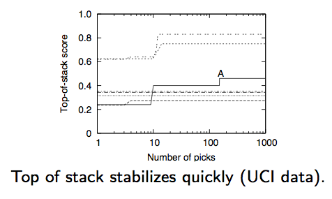
- N=2: try to extend old ideas to new ones;
- N=1; restore old rules
- Usually, N=2 but sometimes N=1. Reflective learning: try to learn new things but sometimes review old things.
- Learn according to domain-specific criteria
- Anytime learning:
- The stack can be a persistent storage for the current state of the inference.
- The stack can be saved, and restored at a later time.
- Anomaly detection:
- If the stack was stable, then top-of-stack starts changing dramatically, then something has changed.
- Temporal learning
- By occasionally using N=1, the learner can revise old knowledge.
- Distributed learning
- Every agent gets their own stack.
- When learners pass each other, one stack of rules gets poured into the others.
- If the other agent's rules are any good, they will rise to the top-of-stack. Otherwise, they'll get buried.