| [ << ] | [ < ] | [ Up ] | [ > ] | [ >> ] | [Top] | [Contents] | [Index] | [ ? ] |
Like tree search, but with a *visited* list that checks if some state has not been reached before.
Visited can take a lot of memory
Best-first search of graph with a *visited* list where states are sorted by "g+h"
Important: proof of A*’s optimality requires that h(x) is an under-estimate cost from "x" to goal
Standard implementation:
For example: http://upload.wikimedia.org/wikipedia/commons/5/5d/AstarExample.gif.
Local search employs the idea that a given solution S may be improved by making small changes. Those solutions obtained by modifying solution S are called neighbors of S.
The local search algorithm starts with some initial solution and moves from neighbor to neighbor as long as possible while decreasing the objective function value. The main problem with this strategy is to escape from local minima where the search cannot find any further neighborhood solution that decreases the objective function value.
Different strategies have been proposed to solve this problem, one of which is tabu search. Tabu search allows the search to explore solutions that do not decrease the objective function value only in those cases where these solutions are not forbidden.
This is usually obtained by keeping track of the last solutions in term of the action used to transform one solution to the next. When an action is performed it is considered tabu for the next T iterations, where T is the tabu status length. A solution is forbidden if it is obtained by applying a tabu action to the current solution.
The Tabu Search metaheuristic has been defined by Fred Glover (see Glover, F. “Future paths for integer programming and links to artificial intelligence”, Comp. Oper. Res., Vol. 13, pp. 533-549, 1986). The basic ideas of TS have also been sketched by P. Hansen (Hansen, P. “The steepest ascent mildest descent heuristic for combinatorial programming”, Congress on Numerical Methods in Combinatorial Optimization, Capri, Italy, 1986).
k := 1
Generate initial solution s
Repeat
    N(s)       :=  neighbours of s
    T(s)       :=  members of N(s) that are tabu at time k
    A(s)       :=  maybe, add in some stuff
	Candidates :=  N(s) - T(s) + A(s)
    Find the best s’ in candidates that maximizes f(s')
    Memorize s’ if it improves the previous best known solution
    s := s’
    k := k+1.
Until some stop critieria
Also, regarding the aspirant set:
Applications
There is a great variety of real-world problems that can be solved by Tabu Search. Representative areas include, but are not limited to:
Consider a function f(x1,x2,x3,...) with inputs x1,x2,x3,... and returns values u1,u2,u3,....
A search for inputs that maximizes all of u1,u2,u3,... may be non-linear in nature (e.g. improvements to u1 might hurt u2; e.g. the cheaper car does not run as fast).
One way to approach this non-linear problem is to randomly generate inputs, then study the results in utility space; i.e. an N-dimensional plot (one dimension for each utility) which contains a utopia point (where are utilites are at their best). Note that is this space, each point shows some set of inputs generated by some inputs.
e.g. from Schmidt M., Lipson H. (2009) "Distilling Free-Form Natural Laws from Experimental Data," Science, Vol. 324, no. 5923, pp. 81 - 85. (see supplemental materials)

A key concept in utility space is Pareto dominiation.
Connection to tabu search:
That’s a simple way to connect this two ideas. But there are better.
NSGA-II: one of the better search mutli-criteria search tools.
So if the above methods are all standard, the enemy knows them too.
Q1: How can you reason about the enemy reasoning about your reasoning?
A1: MinMax trees
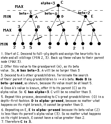
Q2: How you do the above faster?
A2: Alpha-beta pruning
See http://www.ocf.berkeley.edu/~yosenl/extras/alphabeta/alphabeta.html
Note that:
For example (from Wikipedia):
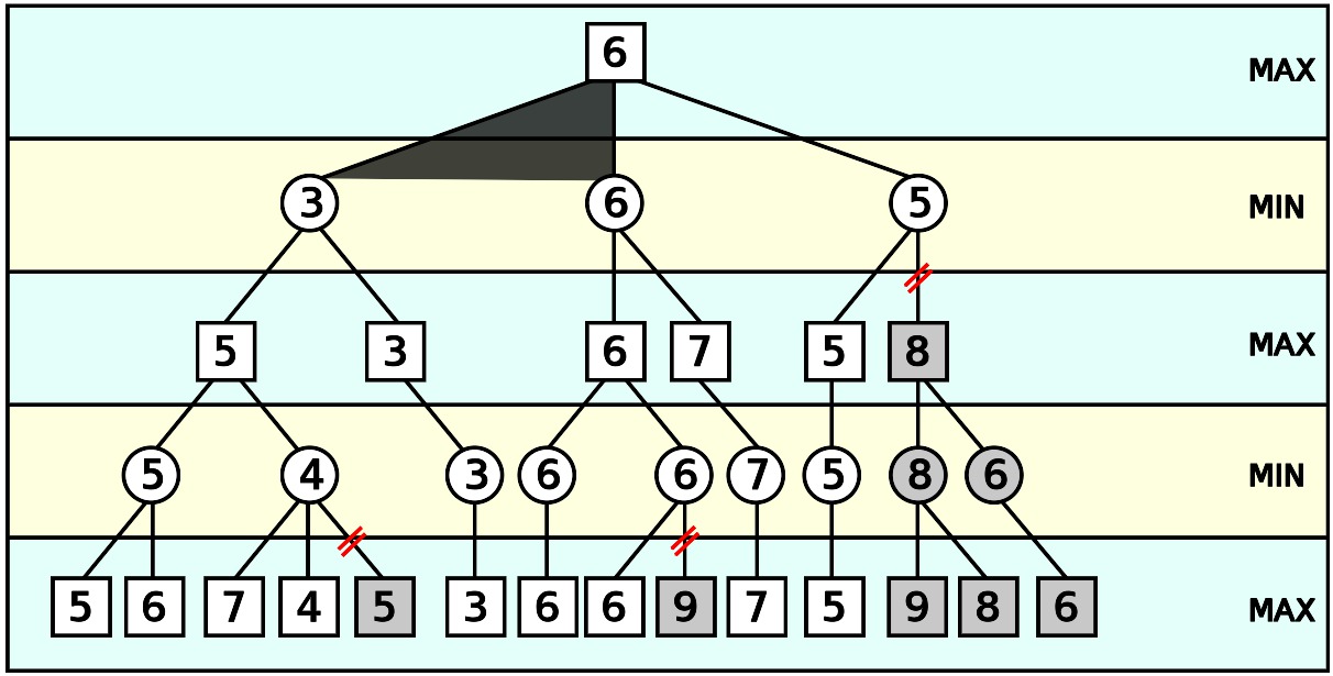
The grayed-out subtrees need not be explored (when moves are evaluated from left to right), since we know the group of subtrees as a whole yields the value of an equivalent subtree or worse, and as such cannot influence the final result. The max and min levels represent the turn of the player and the adversary, respectively.
To guarantee that this algorithm returns a move, we can start alpha with -infinity (the best you can do is lose) and beta with infinity (the worst your opponent can do is to let you win), and update these values as we examine more nodes.
(* Initial call *)
alphabeta(origin, depth, -infinity, +infinity, MaxPlayer)

function alphabeta(node, depth, α, β, Player)
    if  depth = 0 or node is a terminal node
        return the heuristic value of node
    if  Player = MaxPlayer
        for each child of node
            α := max(α, alphabeta(child, depth-1, α, β, not(Player) ))
            if β ≤ α
                break                             (* Beta cut-off *)
        return α
    else
        for each child of node
            β := min(β, alphabeta(child, depth-1, α, β, not(Player) ))
            if β ≤ α
                break                             (* Alpha cut-off *)
        return β
How effective is alpha-beta pruning? It depends on the order in which children are visited. If children of a node are visited in the worst possible order, it may be that no pruning occurs. For max nodes, we want to visit the best child first so that time is not wasted in the rest of the children exploring worse scenarios. For min nodes, we want to visit the worst child first (from our perspective, not the opponent’s.) There are two obvious sources of this information:
A static evaluator function can be used to rank the child nodes Previous searches of the game tree (for example, from previous moves) performed minimax evaluations of many game positions. If available, these values may be used to rank the nodes. When the optimal child is selected at every opportunity, alpha-beta pruning causes all the rest of the children to be pruned away at every other level of the tree; only that one child is explored. This means that on average the tree can searched twice as deeply as before: a huge increase in searching performance.
Finally, there is a common illusion that we first generate a n-ply minmax tree and then apply alpha-beta prune. No, we generate the tree and apply alpha-beta prune at the same time (otherwise, no point).
Strangely, order may not matter. Rather than struggle with lots of tricky decisions,
For example:
Stochastic search: randomly fiddle with current solution
Local search: . replace random stabs with a little tinkering
Some algorithms just do stochastic search (e.g. simulated annealing) while others do both (MAXWALKSAT)
This stochastic tree search can be readily adapted to other problem types.
Eg#1: scheduling problems

Eg#2: N-queens with the lurch algorithm. From state "x", pick an out-arc at random. Follow it to some max depth. Restart.
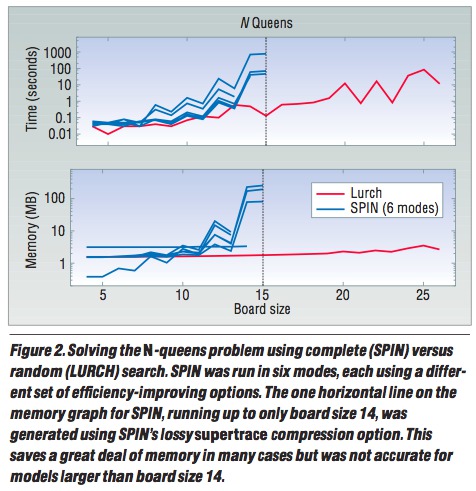
Note: subsequent research found numerous better variants of the at IJCAI’95, AAAI’96, and in 2002.
Q: Why does Isamp work so well. work so well?
S. Kirkpatrick and C. D. Gelatt and M. P. Vecchi Optimization by Simulated Annealing, Science, Number 4598, 13 May 1983, volume 220, 4598, pages 671680,1983.
s := s0; e := E(s)                     // Initial state, energy.
sb := s; eb := e                       // Initial "best" solution
k := 0                                 // Energy evaluation count.
WHILE k < kmax and e > emax            // While time remains & not good enough:
  sn := neighbor(s)                   //   Pick some neighbor.
  en := E(sn)                          //   Compute its energy.
  IF    en < eb                        //   Is this a new best?
  THEN  sb := sn; eb := en             //     Yes, save it.
  FI
  IF random() > P(e, en, k/kmax)       //   Should we move to it?
  THEN  s := sn; e := en               //     Yes, change state.
  FI
  k := k + 1                           //   One more evaluation done
RETURN sb                              // Return the best solution found.
Note the space requirements for SA: only enough RAM to hold 3 solutions. Very good for old fashioned machines.
But what to us for the probability function "P"? This is standard function:
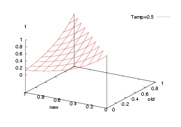
FUNCTION P(old,new,t) = e^((old-new)/t)
Which, incidentally, looks like this...
Initially (t=0):
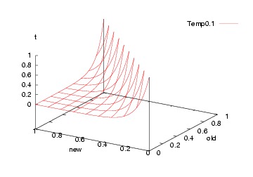
Subsequently (t=0.5):
Finally (t-1):
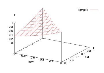
That is, we jump to a worse solution when "random() > P" in two cases:
Note that such crazy jumps let us escape local minima.
Kautz, H., Selman, B., & Jiang, Y. A general stochastic approach to solving problems with hard and soft constraints. In D. Gu, J. Du and P. Pardalos (Eds.), The satisfiability problem: Theory and applications, 573586. New York, NY, 1997.
State of the art search algorithm.
FOR i = 1 to max-tries DO
  solution = random assignment
  FOR j =1 to max-changes DO
    IF    score(solution) > threshold
    THEN  RETURN solution
    FI
    c = random part of solution
    IF    p < random()
    THEN  change a random setting in c
    ELSE  change setting in c that maximizes score(solution)
    FI
RETURN failure, best solution found
This is a very successful algorithm. Here’s some performance of WALKSAT (a simpler version of MAXWALKSAT) against a complete search

You saw another example in the introduction to this subject. The movie at right shows two AI algorithms t$ solve the "latin’s square" problem: i.e. pick an initial pattern, then try to fill in the rest of the square with no two colors on the same row or column.

Link: http://unbox.org/wisp/var/timm/09/ai/share/img/latin.mov
This stochastic local search kills the latin squares problem (and, incidently, many other problems).
GAs = mutate bit-strings
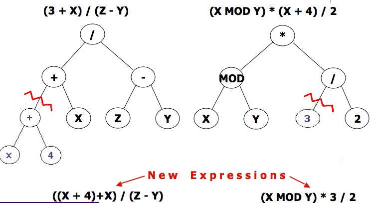
GPs = mutate parse trees of programs
The dream:
Take a herd of variants on a program
GP= mutation of program structure - Special form of GA (genetic algorithms)

Single point crossover (One random crossover point)
before                after
--------------------  --------------------
11111111111111111111  11111111110000000000
00000000000000000000  00000000001111111111
Two point crossover (Two random crossover points)
before                after
--------------------  --------------------
11111111111111111111  11111000001111100000
00000000000000000000  00000111110000011111
Uniform crossover (Probabilistic bit selection)
before                after
--------------------  --------------------
11111111111111111111  11100100111100101001
00000000000000000000  00011011000011010110
Q: Why Mutate?
Approaches
e.g.  order changing
before                after
--------------------  --------------------
11111111111111111111  11100100111100101001
00000000000000000000  00011011000011010110

e.g. adding subtracting

(1.12 3.65 3.86 4.31 5.21) ⇒ (1.12 3.65 3.73 4.23 5.21)
And why stop at bit strings?
Recommended Settings
All generalities are false. But, just to get you started:
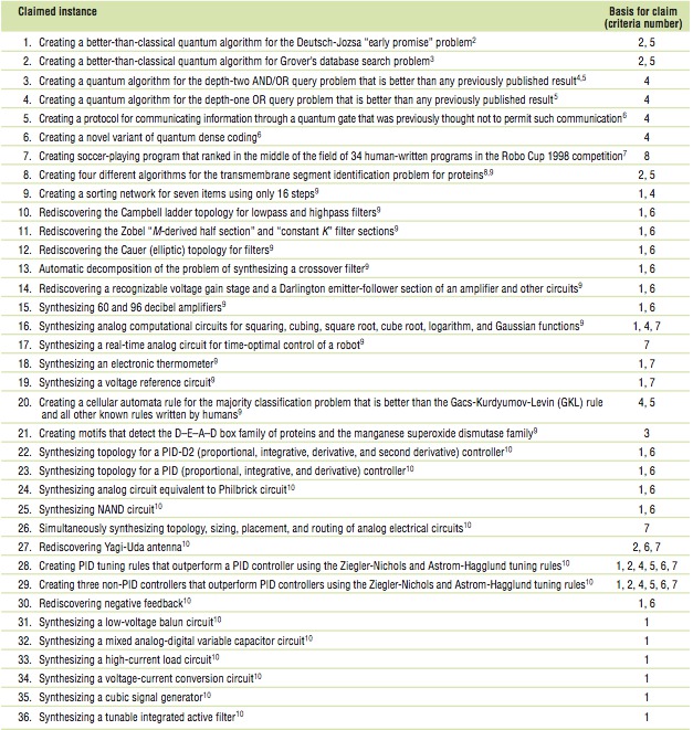
Koza, John R., Keane, Martin A., and Streeter, Matthew J. 2003c. What’s AI done for me lately? Genetic programming’s human-competitive results IEEE Intelligent Systems. Volume 18. Number 3. May/June 2003. Pages 25-31.
Automatic synthesis of computer programs for 21 "human-competitive", previously patented inventions:

Koza lists 36 "human-competitive" results (including the above patents):
| [ << ] | [ < ] | [ Up ] | [ > ] | [ >> ] | [Top] | [Contents] | [Index] | [ ? ] |
This document was generated on March 1, 2011 using texi2html 5.0.